How do you know a fine-tuned AI model is actually better?

You measure it. Hold out a portion of the client's real examples so the model never sees them during training, score the plain base model on those held-out questions first, fine-tune, then score again on the identical questions with identical scoring. The difference is the lift. Because the only thing that changed is the fine-tune, the improvement is attributable to it.

Does fine-tuning actually improve accuracy, or is the base model already good enough?

It depends on the task and, critically, on how much data you have. On a public benchmark of 510 lawyer-annotated commercial contracts, a base Qwen3-4B extracted short contract fields at 62.2% accuracy. Fine-tuned on 396 examples it reached 83.5-85.4%, a lift of 21.3 to 23.2 points across three runs. The same model trained on only 48 examples produced a lift inside the noise floor, so the amount of data was the deciding factor rather than the model's ceiling.

How much of our own data do we need to fine-tune a model?

Fewer examples than most people expect, but more than a handful. In our contract-extraction measurements, 48 training examples produced no measurable improvement while roughly 400 produced a 22-point gain. The honest answer for any specific case is that it depends on how varied and how consistent the examples are, which is what a paid readiness assessment measures on the client's own corpus.

Why can't you just use a public AI benchmark score?

Public benchmarks measure general ability on standardised tests, not your work. A model that scores well in the abstract can still be mediocre at reading your contracts or following your policies. Public benchmarks are also increasingly targeted during training, so a high score can reflect test preparation as much as capability. The only benchmark that answers your question is built from your own tasks.

Research record 21 of 39

Depth Does Not Add Stages

By Joshua Bolick, Awareness Software Group ~11 min read August 2026

Ongoing research. This is an experimental result from active work, not a settled conclusion. The numbers are what we measured and the method is described so you can judge it, but the programme is still running and later experiments may revise what it means. More about this programme.

In plain English

What we asked. Stacking layers is how models are usually made more capable. We wanted to know whether the layers of a deep model learn one after another, each waiting on the one below, or whether they all change at once. If they took turns, you could in principle train them on separate schedules and save effort.

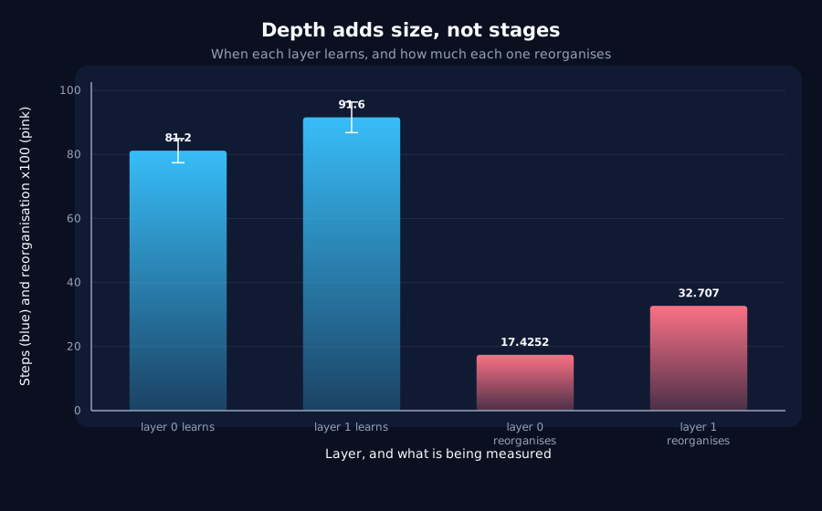
What we found. They move together. The deeper layer does consistently reach its moment slightly after the shallower one, in every run we did, but only by about ten steps when each layer takes roughly sixty steps to make the change. That is one event seen twice rather than two stages. What did differ is how much each layer reorganises itself: the deeper layer changes almost twice as much as the shallower one.

Why it matters. The scheduling idea loses its motivation, which is the useful half. The other half matters more for our own past work: every earlier result in this programme used a single-layer model, and it now turns out the effect we study is stronger nearer the output. So those earlier results were measuring the deep end all along, which is a caveat we have added to them. Getting to any of this took three attempts, because our measuring instrument was broken in a way that produced no result rather than a wrong one.

The rest of this page is the technical record: the design, every number, and the limits. It is written for a reviewer, and you do not need it to have understood the result above.

New here? How to read a research record

Start at the verdict. Every record states, before the experiment was run, what result would have made us abandon the idea. That is the "kill test". Then it says whether the test fired. Nothing gets reinterpreted after the fact.
Numbers in square brackets are uncertainty. 23.4 [18.1, 28.7] means our best estimate is 23.4 and the true value is probably somewhere in that range. If a range includes zero, we cannot claim an effect.
Negative results are kept. Roughly half of what is published here says an idea did not work, including several of our own. Those pages are not failures, they are the output. Work that only publishes what worked is not measuring anything.
Read the Limits section. Every record ends with what it does not show. It is the most honest part of any experiment and usually the shortest.
Pro tip: the figures near the top are designed to carry the result on their own. If you read nothing else, read the caption under each one, which says what it shows and what to take from it.

EXPLORATORY. Not a preregistered study. Local CPU, 28 training runs, no GPU, no cost.

Program v2 tier 4, item E6. Decisive computation: analysis/depth_stages.py. Output: analysis/depth_stages.json. Reproduce with python analysis/depth_stages.py in about forty minutes on a throttled laptop CPU.

The question

Everything recorded in this programme is single-layer. E6 asks whether depth adds temporal structure: in a deep GRU, does each layer learn at its own moment, later layers waiting on earlier ones, or do they all move together?

**Depth adds size, not stages.** A two-layer model, with each layer measured separately. The blue bars are the step at which each layer's internal state starts carrying the answer, with 95% confidence intervals across five runs. The pink bars are how much each layer's state reorganises while that happens, scaled up a hundredfold so both fit on one axis. The two blue bars are close together: the deeper layer does lag the shallower one, consistently, but only by about ten steps when each layer takes roughly sixty steps to make the change. That is not two stages, it is one event seen twice, so the idea of scheduling training layer by layer loses its motivation. The pink bars are the surprise. The deeper layer reorganises almost twice as much as the shallower one, so the effect this project studies is not spread evenly through a model. It concentrates near the output, which is where every earlier single-layer result was measuring.

Kill test, from docs/research-program-v2.md: all layers move within a few steps of each other. Then depth adds parameters but no temporal structure, and per-layer scheduling ideas die cheaply.

Three instrument failures before a number

This record is as much about what it took to measure as about what was measured, because the first two attempts produced nothing and both were the instrument rather than the model.

Layer-resolved capture did not exist. The backlog said it did. capture_representations returned the same three keys at depths 1, 2 and 3, so an intermediate layer could not be read at all. Fixed in the platform: capture now emits recurrent_l0, recurrent_l1, … verified against the stacked module's own output.
The probe was reading the wrong thing. The model's readout is output(final_norm(hidden)), a LayerNorm, then a linear map, and LayerNorm rescales each token individually, which no linear map can undo. A probe fitted to the raw pre-norm state is structurally incapable of matching the model, and it came out 0.43–0.52 below it in every run. Standardising each layer's state per token before fitting lifted the deepest layer's probe from 0.53 to 0.94 against a model at 0.99.
The instrument check was itself too strict. It required every layer's probe to reach the model's accuracy. That target is known-achievable only at the deepest layer, because the model achieves it from there. At an intermediate layer a low ceiling is not a broken probe: it is what depth is for, and the check as written would have discarded every run for precisely the behaviour the study exists to measure.

The learning rate is screened per depth on three seeds excluded from measurement, taking the fastest rate that transitions on every screening seed. A one-seed screen picked a rate that then failed in all five measurement seeds: one seed cannot tell a fast rate from an unstable one.

Depth 2: the layers move together

Screened rate 0.008, 5 of 5 seeds measurable.

Layer	Transition	Own width	Expansion
`recurrent_l0`	`81.2` `[77.4, 85.0]`	`71.2`	`0.1743`
`recurrent_l1`	`91.6` `[86.8, 96.4]`	`50.0`	`0.3271`


Stagger between layers	`10.4` steps
A single layer's own transition width	`60.6` steps
Ratio	`0.17` `[0.09, 0.26]`

The kill test fires. By D2's criterion, reused unchanged, a stagger only counts as stage-wise if it exceeds the width of a single layer's own transition. Here it is a sixth of it, with the whole interval well below 1. Depth adds parameters but no temporal structure, and per-layer scheduling ideas die cheaply.

The honest complication

The stagger is small but not random: the deeper layer transitions later in 5 of 5 runs, and the two intervals ([77.4, 85.0] and [86.8, 96.4]) do not overlap.

So there is a consistent ordering. It is simply far too small, against how long each layer takes to cross, to call the layers separate stages. A record reporting the ordering without the width would have claimed stage-wise learning on a 10-step lag inside a 60-step transition. Both facts belong in the result.

The expansion is not global

The backlog's second question has a cleaner answer than its first. The expansion nearly doubles with depth: 0.1743 at layer 0 against 0.3271 at layer 1.

So the phenomenon this programme has been studying is not uniform across a model's depth. It concentrates in the layer nearest the readout. Every single-layer result in this programme has, by construction, been measuring the equivalent of layer 1, the deep end, which is the more affected one. That is a scope note worth carrying into every earlier record.

Depth 3: not measurable at this budget

All five measurement seeds failed to transition within 520 steps, at a rate where all three screening seeds transitioned at step 111, and where every rate tried solved 3 of 3 on the screen.

That gap: 3 of 3 against 0 of 5, on the same settings, is a finding rather than a failed run. Depth-3 training on this task is seed-fragile at the rates that make depth 2 work. The screen could not transfer, which is exactly what a screen is supposed to warn about, and it did.

What this does not establish: the measurement seeds were only tried at the screened rate. They may well transition at a lower one. Whether depth 3 is genuinely fragile or simply needs a rate the screen did not choose is untested, and is the natural follow-up.

Verdict

Depth 2 layers move together. Ratio 0.17 [0.09, 0.26], kill test fires, per-layer scheduling ideas die cheaply.
The ordering is real and immaterial: consistent in 5 of 5 runs, non-overlapping intervals, and a sixth of a single layer's own transition width.
The expansion is depth-dependent, roughly doubling from layer 0 to layer 1, which scopes every single-layer result in this programme.
Depth 3 is unmeasured, and its screen-to-measurement gap is the informative part.

Limits

One task, one width, five seeds, AdamW, and only two depths measured with one of those failing.
Timing comes from a ridge decode probe, which is a linear instrument. A layer could reorganise in a way a linear readout cannot see, and would then appear not to move.
Layer 0's probe ceiling is far below layer 1's, which is expected and is itself uninterpreted here: it says the answer is not linearly decodable early, not that layer 0 is doing nothing.
The expansion endpoint is a max-minus-baseline quantity, which the programme's standing rule says is positive under noise by construction. The comparison between layers is the claim; neither layer's absolute value should be quoted alone.
Depth is where this task runs out. A three-layer model on a synthetic delayed-copy task is close to the point where the setup stops being able to answer, and the deeper question, whether any of this holds at real width and depth, is not answerable on a throttled laptop.

Terms on this page

Every piece of vocabulary this record uses, in plain language. Generated from the text above, so it cannot drift out of step with it.

accuracy: The fraction of answers a model gets right on questions it was not trained on.
AdamW: A widely used training algorithm that adapts how big a step it takes for each individual parameter. The default in most modern AI training.
baseline: The thing you compare against. A result without one is not a result.
GRU: Gated Recurrent Unit. A compact design for processing sequences one item at a time, with internal switches controlling what it keeps in memory.
kill test: A condition written down before running the experiment that says what result would make us abandon the idea. Fixing it in advance is what stops a disappointing result being reinterpreted as an encouraging one.
learning rate: How big a step training takes each time it updates the model. Too small and nothing happens; too big and it never settles.
parameters: The adjustable numbers inside a model. Training is the process of setting them. Model size is usually quoted as a count of these.
probe: A small separate model trained to read information out of a bigger model's internals, used as a measuring instrument rather than as a product.
seed: The number that fixes all the randomness in a training run. Same seed, same run. Running several seeds is how you tell a real effect from a lucky one.
width: How many internal numbers a model uses at each layer. The usual way we vary model size in these experiments.

About this record. This page is the write-up of an experiment we ran ourselves. Every number on it comes from a run we recorded, and the script that produced each one is named in the text above. We publish these results and the data behind them here, including the ones that went against what we expected.

Why we do this. The same care shown above is what we apply to client work. We build custom AI models that you own and run yourself, using our own platform, and the reason we publish research like this is that a model is only worth what its evaluation is worth. If a supplier cannot show you the experiments that went against them, you cannot check the ones that went their way.

All research from this programme →