How do you know a fine-tuned AI model is actually better?

You measure it. Hold out a portion of the client's real examples so the model never sees them during training, score the plain base model on those held-out questions first, fine-tune, then score again on the identical questions with identical scoring. The difference is the lift. Because the only thing that changed is the fine-tune, the improvement is attributable to it.

Does fine-tuning actually improve accuracy, or is the base model already good enough?

It depends on the task and, critically, on how much data you have. On a public benchmark of 510 lawyer-annotated commercial contracts, a base Qwen3-4B extracted short contract fields at 62.2% accuracy. Fine-tuned on 396 examples it reached 83.5-85.4%, a lift of 21.3 to 23.2 points across three runs. The same model trained on only 48 examples produced a lift inside the noise floor, so the amount of data was the deciding factor rather than the model's ceiling.

How much of our own data do we need to fine-tune a model?

Fewer examples than most people expect, but more than a handful. In our contract-extraction measurements, 48 training examples produced no measurable improvement while roughly 400 produced a 22-point gain. The honest answer for any specific case is that it depends on how varied and how consistent the examples are, which is what a paid readiness assessment measures on the client's own corpus.

Why can't you just use a public AI benchmark score?

Public benchmarks measure general ability on standardised tests, not your work. A model that scores well in the abstract can still be mediocre at reading your contracts or following your policies. Public benchmarks are also increasingly targeted during training, so a high score can reflect test preparation as much as capability. The only benchmark that answers your question is built from your own tasks.

Research record

What a Unit of Training Effort Buys

By Joshua Bolick, Awareness Software Group ~15 min read August 2026

Ongoing research. This is an experimental result from active work, not a settled conclusion. The numbers are what we measured and the method is described so you can judge it, but the programme is still running and later experiments may revise what it means. More about this programme.

Part of a bigger question: Which parts of a model actually matter? – The parts that move most are not the parts that matter, and no single component is required -- the model routes around every freeze. What a part is worth shows up only when you remove it.

In plain English

What we asked. Training a model means nudging millions of numbers, over and over. Not all of those nudges are worth the same: shifting one part of a model can change its behaviour a lot, while shifting another part by the same amount barely changes anything. If the valuable nudges were concentrated somewhere -- in particular parts, or at particular times -- you could spend your money there and skip the rest. We wanted to know whether they are.

What we found. They are concentrated by place, and not at all by time. The best-placed group of a model's internals returns about sixteen times as much change in behaviour, per unit of adjustment, as the worst-placed one. But two checks took most of that finding away again. Measured on a model that has never been trained, the gap is seventeen times -- so the unevenness is built into the design, not something training produces. And the apparent surge of useful work at the moment a model suddenly improves turns out to be smaller than the same measurement taken at a moment picked at random.

Why it matters. Two things are worth taking from this. The first is that we did not invent the measuring instrument. Another group published it, and we ran it side by side with an exact calculation that is only possible because our models are tiny. It agreed, and the small disagreement shrank in exactly the way random noise does when you take more samples, which is how you tell a noisy instrument from a broken one. Importing somebody else's tool and checking it against ground truth is cheap, and it is the difference between using a result and trusting it. The second is the control. Comparing the moment of learning against early training showed every part of the model earning three to four times more, which reads as a discovery. Comparing it against a randomly chosen moment showed the random moment doing better. The quantity just climbs all the way through training, so anything late beats anything early. This is now the fourth time in this project that a control has turned an apparent event into an ordinary trend, and it is the single most repeated lesson in our archive.

The rest of this page is the technical record: the design, every number, and the limits. It is written for a reviewer, and you do not need it to have understood the result above.

New here? How to read a research record

Start at the verdict. Every record states, before the experiment was run, what result would have made us abandon the idea. That is the "kill test". Then it says whether the test fired. Nothing gets reinterpreted after the fact.
Numbers in square brackets are uncertainty. 23.4 [18.1, 28.7] means our best estimate is 23.4 and the true value is probably somewhere in that range. If a range includes zero, we cannot claim an effect.
Negative results are kept. Roughly half of what is published here says an idea did not work, including several of our own. Those pages are not failures, they are the output. Work that only publishes what worked is not measuring anything.
Read the Limits section. Every record ends with what it does not show. It is the most honest part of any experiment and usually the shortest.
Pro tip: the figures near the top are designed to carry the result on their own. If you read nothing else, read the caption under each one, which says what it shows and what to take from it.

EXPLORATORY. Not a preregistered study. Local CPU, 6 training runs plus a 3-point estimator sweep, no GPU, no cost.

Program v2 Bucket P, item P2 (import the published function-space measure and price it) and its parent O2 (function-space work per FLOP). Decisive computation: analysis/function_space_work.py. Output: analysis/function_space_work.json. Reproduce with python analysis/function_space_work.py in about eight minutes on a throttled laptop CPU; --reuse re-derives every endpoint from the saved series without retraining.

The question, and why it matters now

Program v1 closed because reshaping a model's activation coordinates is free at every width, difficulty, subspace and weight tested. That negative was about coordinates. It never measured a single update by its effect on the function the model computes, which is a different object: two updates of identical size can move the model's outputs by wildly different amounts, and only the second kind is buying anything.

**Where a unit of training effort actually lands.** A training step nudges every part of a model, but the parts are not equally worth nudging. Each bar is one group of the model's weights, and its height is how much the model's output actually moved per unit of movement in those weights. Taller means the same effort bought more change. The best-placed group returns about sixteen times what the worst-placed one does, so training effort is very unevenly rewarded. The catch is in the next figure's companion check: measured on a model that has not been trained at all, the gap is seventeen times. The unevenness is built into the design of the model, not produced by training it, so there is no moment during training at which to go looking for it.

**The jump is not when the useful work happens.** Measured at the moment a model suddenly starts performing, every part of it appears to be earning three to four times what it earned early on. That looks like the jump being where the useful work is. The grey bars are the same measurement taken at a moment chosen at random instead, which is the comparison that decides it. The random moment scores higher than the jump does, not lower. The quantity simply climbs all the way through training, so any late moment beats an early one and the jump is not special at all. Without the grey bars the red bars would have read as a discovery. This is the fourth time in this project that a control has turned an apparent event into an ordinary trend.

B1 and B2 propose measuring that at scale on a GPU. This is the CPU precursor that decides whether they are worth funding, and its instrument is imported rather than invented.

Kill test, fixed before execution: function-space work per unit of parameter motion is flat across layers and across training. If a unit of motion buys the same output change wherever and whenever it is spent, there is nothing uneven to exploit.

The instrument, and why we ran two of them

Function-Space Learning Rates (arXiv 2502.17405) defines, for parameter tensor l, the root-mean-square change in the model's outputs caused by that tensor's update alone, and estimates it without the N x K backward passes the definition implies: draw a random w, form the scalar projection phi of the outputs against it, and take one backward pass, which yields every tensor at once.

Our models have 17,280 parameters, so we can compute the quantity exactly, apply only that tensor's update to the live model, run one forward, take the RMS difference in the logits. That is not a second approximation; it is the thing the estimator approximates, including the higher-order terms the first-order expansion drops. Running both is the whole point of importing something.

The import checks out. At 6 draws the estimator sits 23.9% [23.0, 24.7] away from the exact quantity, which looks alarming until it is swept: 0.2269 at 6 draws, 0.1162 at 24, 0.0708 at

That is Monte Carlo noise falling as one over the square root of the draws, not a bias, a

sixteen-fold increase in draws predicts a four-fold reduction and delivers 0.227 -> 0.057 against an observed 0.071. The published estimator is unbiased here, and its accuracy is an ordinary accuracy-for-compute trade.

Anchor

The transition reproduces M3 exactly: 86.7 [82.4, 91.0] against the published [82.4, 91.0], compared as intervals rather than as a point in an interval. The anchor is computed in the committed script, not asserted in this text.

What we found

The work is very uneven across layers, and it was uneven before training started

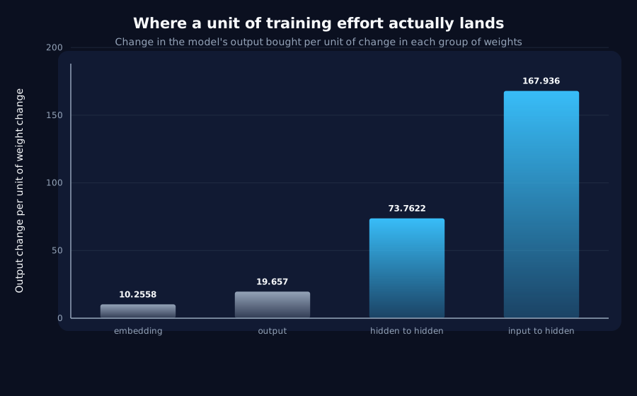
Late in the run, output change bought per unit of parameter motion:

Group	Work per unit of motion
`embedding`	`10.26` `[9.85, 10.66]`
`input_to_hidden`	`167.94` `[159.14, 176.73]`
`hidden_to_hidden`	`73.76` `[60.56, 86.97]`
`output`	`19.66` `[19.34, 19.98]`

The widest pair differs by 16.38x [15.62, 17.14]. The kill test's first half fails cleanly: this is not flat, and a factor of sixteen is large enough to be worth exploiting.

Then the step-0 control fires. The same ratio measured on the model as initialised, against the very first update before any of it has been applied, is 17.44x [16.53, 18.35]: larger, with an overlapping interval. The unevenness is a property of the architecture and the initialisation. Training does not create it and does not increase it.

The first version of this control took the first measured step instead of step 0. That is ten updates in, and therefore already trained. It gave 16.7x and would have supported the same conclusion by luck; it was wrong for the reason a control exists.

The rise across training is drift, not an event

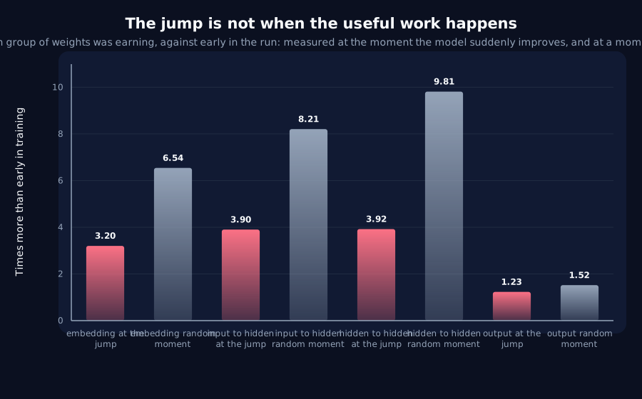
Comparing the transition window against the early run reproduces the shape one would expect from an event: 3.20x, 3.90x, 3.92x and 1.23x for the four groups, intervals well clear of one.

**A random-time-matched window of equal width gives a larger rise**: 6.54x, 8.21x, 9.81x, 1.52x. Comparing the two windows to each other, which is the endpoint that actually isolates the transition, gives:

Group	Transition window over its random-time-matched window
`embedding`	`0.73` `[0.14, 1.32]`
`input_to_hidden`	`0.75` `[0.08, 1.42]`
`hidden_to_hidden`	`0.72` `[-0.00, 1.45]`
`output`	`0.85` `[0.63, 1.07]`

Every interval includes 1.0, and every point estimate is below it. The quantity rises steadily through training, so any late window beats the early run. The transition is not special.

The random window is seeded from the run, not from a constant. The first execution used one constant for every seed, which draws the same step every time: a fixed-schedule arm, not a random-time-matched one (K1).

The instrument's price

At the cadence the paper states, roughly every 100 steps: 10.48% [10.31, 10.66] of the training budget. At this pilot's every-5-steps cadence, 209.7%, a 400-step run has to resolve a transition inside it, so it is measured twenty times more often than the method intends. The exact validation adds a further 80.5%, but that is the audit of the instrument, not the instrument; charging one for the other would overstate the cost by the ratio of the two.

For scale, J7's decode probe cost 55.4% of the budget. This is about a fifth of that, and it is measuring something different.

What this means for B1 and B2

The kill test does not fire, but it does not clear the way either. The work is uneven by a factor of sixteen, which is the precondition B1 and B2 need. But it is uneven at initialisation, and it does not concentrate at the transition.

That splits the two proposals:

Anything that needs to find the moment when useful work concentrates is dead here, by the same random-time-matched control that has now closed several such ideas.
Anything that exploits a fixed, per-layer difference does not need timing at all, and is not touched by this result. That is close to what the source paper's own method does, and it is compatible with this programme's standing rule that the best offline schedule comes first.

Limits

One task, one architecture, one width, one optimiser. The layer grouping is specific to a GRU, and "embedding buys least" may not survive a different input representation.
Biases and norm parameters are folded into their neighbours: at width 48 they carry 384 of 17,280 parameters and a ratio with a near-zero denominator is noise, not signal.
The exact measurement uses the live model rather than a copy, restoring parameters after each group. It is exact for the quantity asked but assumes no state outside the parameters changes, which holds for this model and would need checking for one with running statistics.
work_per_motion is a ratio of two RMS quantities over different-sized tensors. It is comparable across groups by construction and not interpretable as an absolute rate.
The random-time-matched window is drawn once per seed. Six draws characterise the null loosely; a full null distribution would be cheap and is not done here.

Terms on this page

Every piece of vocabulary this record uses, in plain language. Generated from the text above, so it cannot drift out of step with it.

accuracy: The fraction of answers a model gets right on questions it was not trained on.
architecture: The blueprint of a model: what components it has and how they connect. Two models can be the same size and completely different architectures.
GRU: Gated Recurrent Unit. A compact design for processing sequences one item at a time, with internal switches controlling what it keeps in memory.
kill test: A condition written down before running the experiment that says what result would make us abandon the idea. Fixing it in advance is what stops a disappointing result being reinterpreted as an encouraging one.
learning rate: How big a step training takes each time it updates the model. Too small and nothing happens; too big and it never settles.
logits: The raw scores a model produces for each possible answer before they are turned into probabilities.
parameters: The adjustable numbers inside a model. Training is the process of setting them. Model size is usually quoted as a count of these.
probe: A small separate model trained to read information out of a bigger model's internals, used as a measuring instrument rather than as a product.
seed: The number that fixes all the randomness in a training run. Same seed, same run. Running several seeds is how you tell a real effect from a lucky one.
subspace: A slice of a model's internal space: some directions kept, the rest ignored.
width: How many internal numbers a model uses at each layer. The usual way we vary model size in these experiments.

The plain-language version. This page is the record: the design, the numbers and the limits. If you would rather have the story, What a Unit of Training Effort Buys, explained without the jargon, covers the same result for a reader who has never seen a training curve.

About this record. This page is the write-up of an experiment we ran ourselves. Every number on it comes from a run we recorded, and the script that produced each one is named in the text above. We publish these results and the data behind them here, including the ones that went against what we expected.