How do you know a fine-tuned AI model is actually better?

You measure it. Hold out a portion of the client's real examples so the model never sees them during training, score the plain base model on those held-out questions first, fine-tune, then score again on the identical questions with identical scoring. The difference is the lift. Because the only thing that changed is the fine-tune, the improvement is attributable to it.

Does fine-tuning actually improve accuracy, or is the base model already good enough?

It depends on the task and, critically, on how much data you have. On a public benchmark of 510 lawyer-annotated commercial contracts, a base Qwen3-4B extracted short contract fields at 62.2% accuracy. Fine-tuned on 396 examples it reached 83.5-85.4%, a lift of 21.3 to 23.2 points across three runs. The same model trained on only 48 examples produced a lift inside the noise floor, so the amount of data was the deciding factor rather than the model's ceiling.

How much of our own data do we need to fine-tune a model?

Fewer examples than most people expect, but more than a handful. In our contract-extraction measurements, 48 training examples produced no measurable improvement while roughly 400 produced a 22-point gain. The honest answer for any specific case is that it depends on how varied and how consistent the examples are, which is what a paid readiness assessment measures on the client's own corpus.

Why can't you just use a public AI benchmark score?

Public benchmarks measure general ability on standardised tests, not your work. A model that scores well in the abstract can still be mediocre at reading your contracts or following your policies. Public benchmarks are also increasingly targeted during training, so a high score can reflect test preparation as much as capability. The only benchmark that answers your question is built from your own tasks.

Research record

Grow the Model, Save a Quarter

By Joshua Bolick, Awareness Software Group ~11 min read September 2026

Ongoing research. This is an experimental result from active work, not a settled conclusion. The numbers are what we measured and the method is described so you can judge it, but the programme is still running and later experiments may revise what it means.

A note on the language in these records. This is a working laboratory notebook for research into training AI models more cheaply and efficiently, so you will read that an approach did not work, that a result did not hold up, or that one method was worse than another. That is the research doing its job, not a verdict on the engineering we deliver to clients. Ruling an approach out is how the search narrows, and these are the pages that teach us the most: nearly every technique we now rely on came from understanding why something else fell short. Testing our own ideas at least as hard as anyone else's is the point of publishing them. More about this programme and why we run it.

Part of a bigger question: What actually makes training cheaper? – One thing has worked: stopping part of the training early saved about 7% with no loss of quality. Everything else tested has been matched by a simpler or cheaper method -- and in two cases the clever method was only winning because it was quietly being given more.

In plain English

What we asked. Training a small model is cheap but it may never get good enough; training a big one works but costs more. We tried starting small and doubling the model's size twice during training, copying it each time so nothing already learned was lost.

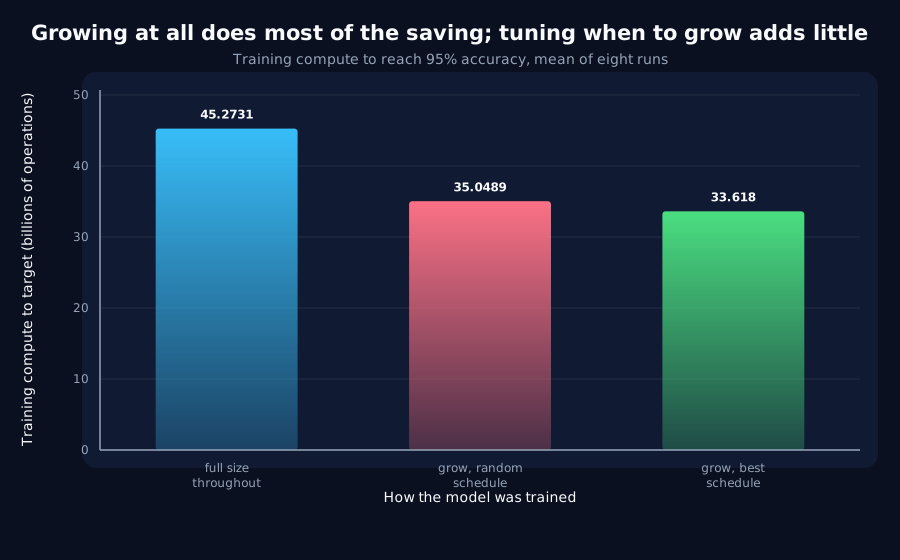
What we found. The growing model reached the target with 26 percent less compute than one trained at full size throughout, and ended slightly more accurate. Models kept small never reached the target. And the exact moments to grow hardly mattered: random timings saved 23 percent, and searching for the best timing added only a little.

Why it matters. In practice: if you are going to train a model to a given size, consider starting smaller and growing it. Do not spend much on tuning when.

The rest of this page is the technical record: the design, every number, and the limits. It is written for a reviewer, and you do not need it to have understood the result above.

New here? How to read a research record

Start at the verdict. Every record states, before the experiment was run, what result would have made us abandon the idea. That is the "kill test". Then it says whether the test fired. Nothing gets reinterpreted after the fact.
Numbers in square brackets are uncertainty. 23.4 [18.1, 28.7] means our best estimate is 23.4 and the true value is probably somewhere in that range. If a range includes zero, we cannot claim an effect.
Results that rule an idea out are kept. Roughly half of what is published here says an approach did not work, including plenty of our own. Those pages are the output, not a shortfall: knowing which direction is a dead end is what lets the next experiment go somewhere better, and most of what we now rely on came out of understanding why something else fell short. Work that only publishes what worked is not measuring anything.
Read the Limits section. Every record ends with what it does not show. It is the most honest part of any experiment and usually the shortest.
Pro tip: the figures near the top are designed to carry the result on their own. If you read nothing else, read the caption under each one, which says what it shows and what to take from it.

EXPLORATORY. Not a preregistered study. Local CPU, 67 training runs (27 schedule-tuning runs on throwaway seeds, 40 measured). The growth method, arms, endpoint and kill test were committed (89bf122) before any run.

Program v2 Bucket O, item O5. Decisive computation: analysis/progressive_width.py. Output: analysis/progressive_width.json. Reproduce with python analysis/progressive_width.py (about an hour on a throttled laptop CPU); --reuse re-derives every endpoint from the saved series.

The question

The literature reports large savings from growing a model during training. This programme's rules say a manoeuvre must beat the best fixed alternative found offline, against a narrow-trained control, with cost counted in compute rather than steps. O5 prices width growth under those rules.

**Starting small and growing reaches the target with a quarter less compute.** Four ways to train the same kind of model on the same task. Three stay one size throughout; the orange line starts a quarter of the size and doubles twice, copying itself so nothing it has learned is lost. *The growing model crosses the target band with about 26% less compute than the full-size one, and the smaller fixed models do not reach it at all in this budget.*

**Growing at all does most of the saving; tuning when to grow adds little.** The compute each approach needed to reach 95% accuracy. The best schedule was found by a search of 27 extra training runs; the random schedule needed no search. *A random growth schedule already saves 23%; the searched-for one saves 26%. The search cost about three thousand times the extra it saves per run.*

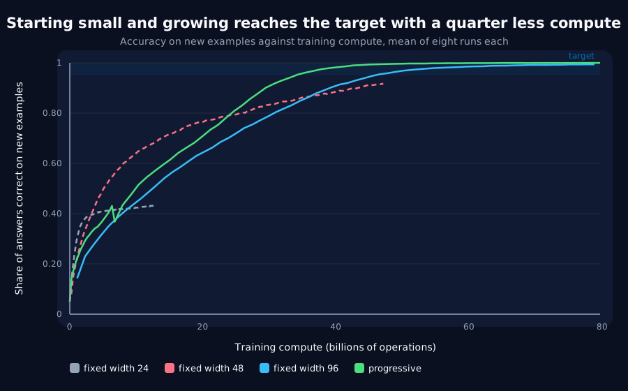
A GRU starts at width 24, doubles to 48 at step s1 and to 96 at step s2, by function-preserving duplication (every unit copied, every weight reading from a copied unit halved, so the logits are unchanged -- checked in code at every growth; LayerNorm statistics are preserved because every value appears twice), then a small perturbation to break the symmetry. The optimiser restarts at each growth. Task: T11's random stream (copy at lag 4), batch 64, rate 0.006, 1500 steps. Endpoint: training FLOPs to held-out accuracy 0.95 (forward-pass FLOPs of the recurrence and readout; the backward pass is a common factor).

Arms on J8's eight receivers: fixed-24, fixed-48, fixed-96; progressive, at the best schedule found offline on three throwaway seeds over nine (s1, s2) pairs; random growth, a schedule drawn per receiver from the same nine.

Kill test, fixed before execution: progressive minus the best fixed width, or progressive minus random growth, has an interval including zero or above it.

Result: the kill test does not fire

Arm	Reached `0.95`	FLOPs to `0.95` (mean)	Final accuracy (step `1500`)
fixed-24	`0/8`	--	--
fixed-48	`1/8`	(`42.3` G, one seed)	`0.917`
fixed-96	`8/8`	`45.3` G	`0.9926`
progressive (grow at `50`, `250`)	`8/8`	`33.6` G	`0.9992`
random growth	`8/8`	`35.0` G	`0.9995`

Paired difference (eight receivers)	FLOPs
progressive minus fixed-96 (the best fixed width)	`-11.7` G `[-13.3, -10.1]`
progressive minus random growth	`-1.4` G `[-2.6, -0.2]`

Growing from width 24 to 96 reaches the target in 26% fewer FLOPs than training at width 96 throughout, and finishes more accurate. The narrow-trained controls cannot reach the target in the budget at all (fixed-48 on one seed of eight), so width 96 is the cheapest fixed option, and the saving is against it.

The schedule barely matters. The best offline schedule beats a randomly drawn one by 1.4 G, an interval that excludes zero but is a sixth of the saving; random growth alone saves 23%.

Pricing the search

The best schedule came from 27 full tuning runs, about 4,200 G of compute, to buy 1.4 G per run over a random schedule. The search costs about three thousand times what it saves per run; it would pay back only over thousands of runs. Growing at any schedule in the grid captures most of the saving with no search at all.

What stands

Kill test does not fire. Progressive width saves 11.7 G [10.1, 13.3] of 45.3 G (26%) against the cheapest fixed width that reaches the target, with higher final accuracy.
Most of it needs no tuning: a random growth schedule from the same grid saves 23%.
This is the first efficiency result in this programme to survive a compute-matched comparison against the cheapest fixed alternative and a random-schedule control. It is one task, one model family and small widths.

Limits

One task (a copy task on a random stream), one rate, widths 24-96, 1500 steps. The growth rule is full duplication (doubling only).
FLOPs count the forward pass of the recurrence and readout; the growth operation, the optimiser restart and evaluation are not counted (all small here).
The tuning grid starts growth by step 200; later growth was not tried.

QUALIFIED 2026-09-27 by O27. Rerun unchanged on a second, slower task (modular sum), no growth schedule in this record's grid reached the target on all three throwaway seeds, and the four runs that did reach it cost more than a fixed width. The grid was built for this record's task's timescale; O28 tests a grid scaled to the second task. Until then the saving here is a one-task result. Text and numbers above unchanged.

Terms on this page

Every piece of vocabulary this record uses, in plain language. Generated from the text above, so it cannot drift out of step with it.

accuracy: The fraction of answers a model gets right on questions it was not trained on.
compute-matched: Comparing two methods by giving them the same amount of computing power rather than the same number of steps. A method that takes twice as long per step should not get twice the compute for free.
GRU: Gated Recurrent Unit. A compact design for processing sequences one item at a time, with internal switches controlling what it keeps in memory.
held-out: Data the model was never trained on, kept back specifically to test it. Scoring a model on data it has already seen measures memorisation, not learning.
kill test: A condition written down before running the experiment that says what result would make us abandon the idea. Fixing it in advance is what stops a disappointing result being reinterpreted as an encouraging one.
logits: The raw scores a model produces for each possible answer before they are turned into probabilities.
seed: The number that fixes all the randomness in a training run. Same seed, same run. Running several seeds is how you tell a real effect from a lucky one.
width: How many internal numbers a model uses at each layer. The usual way we vary model size in these experiments.