How do you know a fine-tuned AI model is actually better?

You measure it. Hold out a portion of the client's real examples so the model never sees them during training, score the plain base model on those held-out questions first, fine-tune, then score again on the identical questions with identical scoring. The difference is the lift. Because the only thing that changed is the fine-tune, the improvement is attributable to it.

Does fine-tuning actually improve accuracy, or is the base model already good enough?

It depends on the task and, critically, on how much data you have. On a public benchmark of 510 lawyer-annotated commercial contracts, a base Qwen3-4B extracted short contract fields at 62.2% accuracy. Fine-tuned on 396 examples it reached 83.5-85.4%, a lift of 21.3 to 23.2 points across three runs. The same model trained on only 48 examples produced a lift inside the noise floor, so the amount of data was the deciding factor rather than the model's ceiling.

How much of our own data do we need to fine-tune a model?

Fewer examples than most people expect, but more than a handful. In our contract-extraction measurements, 48 training examples produced no measurable improvement while roughly 400 produced a 22-point gain. The honest answer for any specific case is that it depends on how varied and how consistent the examples are, which is what a paid readiness assessment measures on the client's own corpus.

Why can't you just use a public AI benchmark score?

Public benchmarks measure general ability on standardised tests, not your work. A model that scores well in the abstract can still be mediocre at reading your contracts or following your policies. Public benchmarks are also increasingly targeted during training, so a high score can reflect test preparation as much as capability. The only benchmark that answers your question is built from your own tasks.

Research record

A Shortcut Only Matters If There Is No Other One

By Joshua Bolick, Awareness Software Group ~15 min read September 2026

Ongoing research. This is an experimental result from active work, not a settled conclusion. The numbers are what we measured and the method is described so you can judge it, but the programme is still running and later experiments may revise what it means.

A note on the language in these records. This is a working laboratory notebook for research into training AI models more cheaply and efficiently, so you will read that an approach did not work, that a result did not hold up, or that one method was worse than another. That is the research doing its job, not a verdict on the engineering we deliver to clients. Ruling an approach out is how the search narrows, and these are the pages that teach us the most: nearly every technique we now rely on came from understanding why something else fell short. Testing our own ideas at least as hard as anyone else's is the point of publishing them. More about this programme and why we run it.

Part of a bigger question: Which parts of a model actually matter? – The parts that move most are not the parts that matter, and no single component is required -- the model routes around every freeze. What a part is worth shows up only when you remove it.

In plain English

What we asked. Three of our earlier results pointed at the same small piece of wiring inside a model, the connection that lets a unit feed its own output back to itself, and they did not obviously agree. One said that wiring is worth a lot. Another said it carries almost nothing. A third pointed out that one of the two designs we use has that connection built in by default. Anyone reading all three in a row would notice the tension.

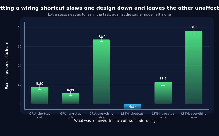
What we found. It turns out they were measuring different things and all three were right. Removing the wiring from the design permanently costs about nine steps of learning. Removing only the part it contributes to a single learning step costs about six, against thirty-four for removing everything else. So the wiring matters for what the model can do, and barely matters for what any one learning step does. Those are separate questions and nobody had measured both on the same models before.

Why it matters. The sharper finding is the comparison between the two designs. Cutting the wiring costs the first design nine steps and costs the second nothing at all, because the second has a separate route that does the same job. That is worth knowing well beyond this experiment: a result about one architecture can fail to carry to another, not because the finding was wrong, but because the second architecture already had another way to get the same thing. We also report the test two ways, because on its strictest reading it says one thing and in the units it actually named it says the opposite, and picking whichever we preferred is a mistake we made a few pages ago and would rather not repeat.

The rest of this page is the technical record: the design, every number, and the limits. It is written for a reviewer, and you do not need it to have understood the result above.

New here? How to read a research record

Start at the verdict. Every record states, before the experiment was run, what result would have made us abandon the idea. That is the "kill test". Then it says whether the test fired. Nothing gets reinterpreted after the fact.
Numbers in square brackets are uncertainty. 23.4 [18.1, 28.7] means our best estimate is 23.4 and the true value is probably somewhere in that range. If a range includes zero, we cannot claim an effect.
Results that rule an idea out are kept. Roughly half of what is published here says an approach did not work, including plenty of our own. Those pages are the output, not a shortfall: knowing which direction is a dead end is what lets the next experiment go somewhere better, and most of what we now rely on came out of understanding why something else fell short. Work that only publishes what worked is not measuring anything.
Read the Limits section. Every record ends with what it does not show. It is the most honest part of any experiment and usually the shortest.
Pro tip: the figures near the top are designed to carry the result on their own. If you read nothing else, read the caption under each one, which says what it shows and what to take from it.

EXPLORATORY. Not a preregistered study. Local CPU, two architectures across four arms over eight seeds, no GPU, no cost.

Program v2 Bucket L, item L6. Decisive computation: analysis/self_connection_reconciliation.py. Output: analysis/self_connection_reconciliation.json. Reproduce with python analysis/self_connection_reconciliation.py in about twenty minutes on a throttled laptop CPU; --reuse re-derives every endpoint from the saved series.

The question

Three records point at the recurrent diagonal and a reader will notice the tension before we do.

**Cutting a wiring shortcut slows one design down and leaves the other unaffected.** Both designs let a unit feed back into itself. We removed that in three ways and timed how much longer each model took to learn. Bars above the line mean slower. "Shortcut cut" removes it from the design permanently. "One step only" removes just the part it contributes to a single learning step. "Everything else" removes all the other wiring instead, as a yardstick for how big these numbers are. Cutting the shortcut costs the first design about nine steps and costs the second nothing at all, because the second has a separate route that does the same job. That settles a disagreement between three of our earlier results: one said this wiring matters, another said it carries almost nothing, and both were right about different things. Whether it matters depends on whether the design has another way to get the same effect, which is a useful thing to know before copying a result from one architecture to another.

G4: at 25% density, block-diagonal sparsity transitions 21 steps before plain random and 13 before random-with-the-diagonal-kept. Self-connections were read as explaining a large share of that.
J3: the leading gradient direction's causal power is 6.5x off-diagonal, +5.3 against +34.5 steps, and the diagonal barely beats a span-random control.
K5: an LSTM's cell state is a self-connection by construction, and the LSTM has the same critical period as the GRU.

Kill test, fixed before execution: at matched energy, the self-connections' causal cost is the same in an LSTM as in a GRU.

Prior recorded in advance: the kill test fires, because J3's result is about where gradient energy sits rather than what the recurrence is made of. That prior was wrong on the literal reading and right on the one the kill test actually asked for. Both are below.

Anchor, enforced in code. J3's GRU numbers reproduce at +5.6 and +33.7 against the published +5.3 and +34.5, both inside one evaluation interval. The script imports J3's own module and exits 2 without interpreting anything if they do not.

Result

Steps to the transition against each architecture's own control. Positive means slower.

Arm	What it removes	`tiny-gru`	`tiny-lstm`
`diagonal`	the leading direction's diagonal component	`+5.6` `[+4.5, +6.8]`	`+11.5` `[+9.4, +13.5]`
`off-diagonal`	the matched off-diagonal component	`+33.7` `[+32.7, +34.7]`	`+38.3` `[+36.4, +40.1]`
`diagonal-severed`	the self-connections, permanently, from init	`+8.9` `[+7.5, +10.3]`	`-2.8` `[-3.7, -2.0]`

Held-out accuracy ends at 0.973 to 0.985 in every cell, so none of this is bought by damaging the model.

The three records never disagreed

G4 and J3 measure different objects, and this is the first run to carry both measurements.

On the same architecture, the same task and the same seeds: severing the self-connections structurally costs +8.9 steps, while removing the leading direction's diagonal component costs +5.6 against +33.7 for its off-diagonal component. The structural contribution is real and it is larger than the dynamic one, and the dynamic one is still 6.0x smaller than the off-diagonal component next to it.

So G4 is right that self-connections matter, J3 is right that the leading direction's power is off-diagonal, and neither statement constrains the other. A structure can be load-bearing for what a model is able to represent while contributing little to the causal power of one direction at one moment. That was assertable before; it is measured now.

K5's aside, made causal

The sharpest number here is the one the kill test did not ask for.

Severing the gate-matrix diagonal costs a GRU +8.9 steps and costs an LSTM -2.8. The intervals are nowhere near each other and the LSTM's sign is negative: it is very slightly faster without them.

That is K5's observation turned into a causal claim. The LSTM has a second route to self-connection that the GRU does not: the cell state carries c_t forward directly, so removing the diagonal of W_hh does not remove the architecture's ability to connect a unit to itself. The GRU has no such route and pays nine steps for losing it.

This is the reconciliation. Self-connections matter, and how much they matter depends on whether the architecture has another way to get them.

The kill test, read two ways, and why both are reported

Literally, on raw intervals, it does not fire. The GRU's diagonal costs +5.6 [+4.5, +6.8] and the LSTM's +11.5 [+9.4, +13.5]. Those do not overlap, so the cost is not "the same".

But the energies are matched within an architecture and not across one, and the kill test says at matched energy. The LSTM's arms strip about 2.2x what the GRU's do, because a fourth gate puts more of the gradient on the diagonal:

	energy removed	steps	steps per unit energy
`tiny-gru` diagonal	`0.1643`	`+5.6`	`34.2`
`tiny-lstm` diagonal	`0.3558`	`+11.5`	`32.2`
`tiny-gru` off-diagonal	`0.1319`	`+33.7`	`255.7`
`tiny-lstm` off-diagonal	`0.4160`	`+38.3`	`92.0`

Per unit of gradient energy removed, the diagonal costs the same in both: 34.2 against 32.2. In the unit the kill test named, it fires.

Q8 is why this paragraph exists rather than a preference. There, I distrusted a preregistered test because of a confound and then preferred an explanation the identical confound protected. The check that makes this different: the confound is unequal energy across architectures, and the normalisation divides by the confounded quantity rather than being shielded by it. The structural arm, which carries the record's actual finding, uses no energy matching at all and is untouched either way. If both of those were false this would be Q8 again.

What stands

G4, J3 and K5 do not disagree. Structure and dynamics are different objects and this is the first run to measure both on the same models.
Self-connections are structurally load-bearing in a GRU, worth +8.9 steps, and not in an LSTM, worth -2.8, because the cell state already provides the connection.
The leading direction's diagonal component is weak in both, 6.0x and 3.3x smaller than the matched off-diagonal component, reproducing J3.
Per unit of energy removed the diagonal costs the same in both architectures, which is the kill test's own unit and is the reading I would quote.

Limits

One task. G4, J3, K5 and this are all delayed-copy, and L7 showed the critical period is a delayed-copy fact. This reconciles three records with each other and extends none of them to another task. That is now the subject of its own bucket (R1), because only 9 of 119 committed pilots have ever run on a second task.
One width (48), one learning rate, one 40-step window taken from J3.
The cross-architecture surgery comparison is not energy-matched, which is stated above rather than buried. The structural comparison has no such issue.
diagonal-severed removes the gate matrix's diagonal only. It does not and cannot remove an LSTM's cell state, which is the whole point of the contrast, but it does mean "severed" means something slightly different in the two architectures. The record says so rather than implying a clean ablation.
Eight seeds, and the LSTM's -2.8 is small. It is clearly separated from the GRU's +8.9, and it should not be read as evidence that severing helps an LSTM.

Terms on this page

Every piece of vocabulary this record uses, in plain language. Generated from the text above, so it cannot drift out of step with it.

accuracy: The fraction of answers a model gets right on questions it was not trained on.
architecture: The blueprint of a model: what components it has and how they connect. Two models can be the same size and completely different architectures.
confound: A second explanation you did not control for. If bigger models both learn faster and score higher, then 'fast learners score higher' may be entirely about size and not about speed.
critical period: A stretch of time during which something has to happen for development to proceed normally. Borrowed from biology, where it describes windows in which a young brain must receive certain input.
evaluation interval: The gap between successive checks of a model during training. It is the smallest difference in timing a measurement can resolve, so two results closer together than one interval cannot be told apart.
gradient: The direction and amount by which each of a model's internal numbers should change to do slightly better. Training is repeatedly following it.
GRU: Gated Recurrent Unit. A compact design for processing sequences one item at a time, with internal switches controlling what it keeps in memory.
held-out: Data the model was never trained on, kept back specifically to test it. Scoring a model on data it has already seen measures memorisation, not learning.
kill test: A condition written down before running the experiment that says what result would make us abandon the idea. Fixing it in advance is what stops a disappointing result being reinterpreted as an encouraging one.
learning rate: How big a step training takes each time it updates the model. Too small and nothing happens; too big and it never settles.
LSTM: Long Short-Term Memory. An older and larger relative of the GRU, also gated, also for sequences.
normalisation: Dividing a measurement by something else to make it comparable across cases. What you divide by is a choice, and it can change the answer as much as the data does.
recurrent: A design that reads a sequence one item at a time, carrying memory forward. The main alternative is attention, which looks at everything at once.
seed: The number that fixes all the randomness in a training run. Same seed, same run. Running several seeds is how you tell a real effect from a lucky one.
width: How many internal numbers a model uses at each layer. The usual way we vary model size in these experiments.