How do you know a fine-tuned AI model is actually better?

You measure it. Hold out a portion of the client's real examples so the model never sees them during training, score the plain base model on those held-out questions first, fine-tune, then score again on the identical questions with identical scoring. The difference is the lift. Because the only thing that changed is the fine-tune, the improvement is attributable to it.

Does fine-tuning actually improve accuracy, or is the base model already good enough?

It depends on the task and, critically, on how much data you have. On a public benchmark of 510 lawyer-annotated commercial contracts, a base Qwen3-4B extracted short contract fields at 62.2% accuracy. Fine-tuned on 396 examples it reached 83.5-85.4%, a lift of 21.3 to 23.2 points across three runs. The same model trained on only 48 examples produced a lift inside the noise floor, so the amount of data was the deciding factor rather than the model's ceiling.

How much of our own data do we need to fine-tune a model?

Fewer examples than most people expect, but more than a handful. In our contract-extraction measurements, 48 training examples produced no measurable improvement while roughly 400 produced a 22-point gain. The honest answer for any specific case is that it depends on how varied and how consistent the examples are, which is what a paid readiness assessment measures on the client's own corpus.

Why can't you just use a public AI benchmark score?

Public benchmarks measure general ability on standardised tests, not your work. A model that scores well in the abstract can still be mediocre at reading your contracts or following your policies. Public benchmarks are also increasingly targeted during training, so a high score can reflect test preparation as much as capability. The only benchmark that answers your question is built from your own tasks.

Research record

Is Learning a Lucky Accident?

By Joshua Bolick, Awareness Software Group ~10 min read August 2026

Ongoing research. This is an experimental result from active work, not a settled conclusion. The numbers are what we measured and the method is described so you can judge it, but the programme is still running and later experiments may revise what it means. More about this programme.

In plain English

What we asked. Training an AI involves a large amount of randomness. We asked whether the sudden moment of learning is the model getting lucky, randomly stumbling into a solution, or whether it was always going to happen.

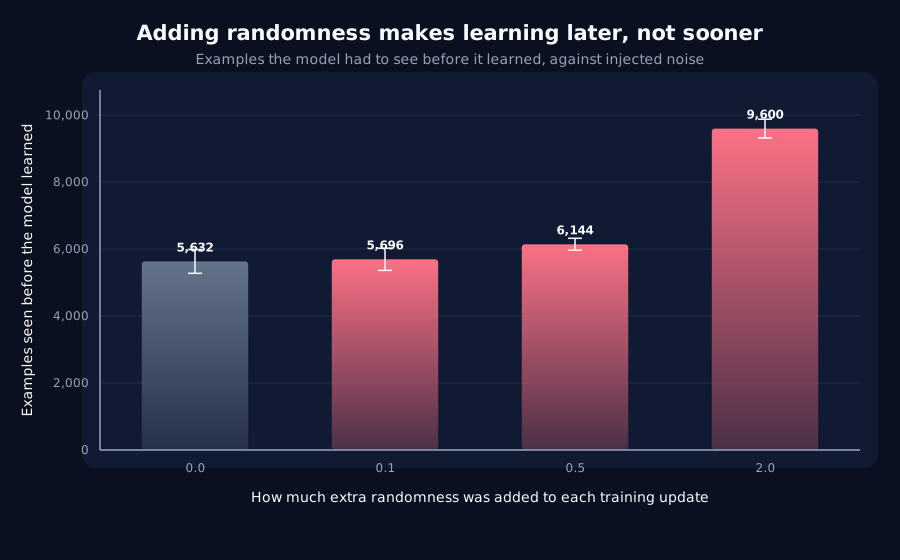
What we found. Not luck, and randomness actively gets in the way. When we injected extra randomness while holding everything else fixed, learning arrived later, not sooner, and the transition smeared out. A separate test that seemed to show randomness helping turned out to be measuring something else entirely.

Why it matters. There was a plausible theory that a model sits stuck until random noise kicks it loose. If that were true, adding noise on purpose would be a training technique. It is not: noise is friction here, not fuel, and that closes off a line of work we had been holding open.

The rest of this page is the technical record: the design, every number, and the limits. It is written for a reviewer, and you do not need it to have understood the result above.

New here? How to read a research record

Start at the verdict. Every record states, before the experiment was run, what result would have made us abandon the idea. That is the "kill test". Then it says whether the test fired. Nothing gets reinterpreted after the fact.
Numbers in square brackets are uncertainty. 23.4 [18.1, 28.7] means our best estimate is 23.4 and the true value is probably somewhere in that range. If a range includes zero, we cannot claim an effect.
Negative results are kept. Roughly half of what is published here says an idea did not work, including several of our own. Those pages are not failures, they are the output. Work that only publishes what worked is not measuring anything.
Read the Limits section. Every record ends with what it does not show. It is the most honest part of any experiment and usually the shortest.
Pro tip: the figures near the top are designed to carry the result on their own. If you read nothing else, read the caption under each one, which says what it shows and what to take from it.

EXPLORATORY. Not a preregistered study. Local CPU, 40 training runs, no GPU, no cost.

Program v2 tier 3, item D7. Decisive computation: analysis/noise_driven.py. Output: analysis/noise_driven.json. Reproduce with python analysis/noise_driven.py in about twenty-five minutes on a throttled laptop CPU. The numbers below reproduced exactly on a second execution.

The question

Is the transition a stochastic escape, the model sitting on a plateau until gradient noise knocks it off, or deterministic optimisation finding a feature that was always reachable?

**Adding randomness makes learning later, not sooner.** Training an AI is a partly random process, and one popular explanation for sudden learning is that the randomness eventually knocks the model out of a rut. If that were right, adding more randomness on purpose should make learning arrive sooner. We added it, holding everything else fixed, and measured how much data the model needed before it learned. The leftmost bar is the untouched control, and the whiskers show the spread across five independent runs. Every increase in randomness made learning take longer, and the strongest setting needed 70% more data than the control while also smearing the moment of learning out over twice the span. Randomness is friction here, not fuel. That rules out the rut-escape explanation, and closes off the idea of deliberately adding noise to speed training up, at least for this kind of model.

The distinction is not academic. A4 proposed kick-style interventions: if noise is what ends the plateau, supplying it deliberately is a training technique. D3 already removed A4's other leg by showing timing is not steerable, so this is the last thing holding that line open.

Kill test, from docs/research-program-v2.md: neither timing nor sharpness responds to noise scale.

Why this ran two arms

The backlog specifies a batch-size sweep at fixed total examples. That design has a confound, and it is a serious one: changing batch size changes three things at once: the gradient noise, the number of optimiser updates, and the effective step size per example. A difference between batch 16 and batch 256 cannot be attributed to noise when the smaller batch also took sixteen times as many steps.

So the batch sweep runs as specified, and a second arm isolates the variable:

Arm A, batch sweep. Fixed total examples (57,600), batch 16 / 64 / 256, plus a full-batch arm over a fixed 1,024-example pool: the noise-free endpoint, possible only because the trainer gained a fixed-dataset mode in tier 1. Timing is reported in examples seen, not steps, because a step means something different in each arm.
Arm B, direct injection. Gaussian noise added to the gradient at fixed batch size, fixed step count and fixed learning rate. Everything except the noise is held constant.

Arm B is decisive; Arm A is the context for it.

Arm A: the confounded sweep, and what it looks like

Arm	Learned	Final accuracy	Transition (examples)	Width (examples)
batch 16	5/5	`0.9899`	`2,560` `[2560, 2560]`	2,112
batch 64	5/5	`0.9942`	`5,632` `[5277, 5987]`	4,224
batch 256	5/5	`0.9894`	`15,360` `[15042, 15678]`	11,571
full batch (1024)	5/5	`0.6558`	`34,202` `[32752, 35651]`	26,829

Read naively this is a large, clean, monotone noise effect: more noise, earlier transition, spanning 219% of the mean. It is also almost entirely the confound. Converting to optimiser steps:

Arm	Transition in examples	Transition in steps
batch 16	2,560	160
batch 64	5,632	88
batch 256	15,360	60
full batch	34,202	33

The ordering reverses. In examples the small batch is 13.4x earlier; in steps the large batch is 4.8x earlier. Neither unit is invariant, but steps is much closer, which is what you would expect if the dominant variable were update count rather than noise.

The full-batch arm also fails to learn the task properly (0.6558 against 0.99), so its transition is measured on a run that never got there. It is reported for completeness and carries no weight.

Arm B: the clean test

Fixed batch 64, fixed steps, fixed learning rate. Only the injected gradient noise varies.

Arm	Learned	Final accuracy	Transition (examples)	Width (examples)
noise x0.0	5/5	`0.9942`	`5,632` `[5277, 5987]`	4,224
noise x0.1	5/5	`0.9937`	`5,696` `[5364, 6028]`	4,160
noise x0.5	5/5	`0.9922`	`6,144` `[5966, 6322]`	4,480
noise x2.0	5/5	`0.9816`	`9,600` `[9319, 9881]`	8,576

Seed-to-seed spread within one arm is 12.6% of the transition point, so a response counts only above that.

Timing moves 58.6%, above the seed spread. The transition responds.
The direction is later: 1.70x at the strongest noise, monotone across all four levels.
Sharpness moves 82.4%, and the transition gets broader, not narrower: width doubles.
The response is threshold-like rather than proportional. x0.1 is indistinguishable from the control and x0.5 barely clears it; nearly all of the effect is at x2.0.

Verdict: the kill test does not fire, and A4 dies anyway

The literal kill test, no response to noise, does not fire. Timing and sharpness both respond beyond seed noise. Reported as a magnitude alone, that reads as support for the stochastic escape picture.

The direction reverses the conclusion. A4 required noise to be what ends the plateau. Injected noise makes the plateau longer and the transition blurrier, monotonically. Noise is not the kick; it is drag on a process that was going to happen anyway.

So:

The transition is not a stochastic escape. Removing noise does not prevent it and adding noise does not trigger it, adding noise delays it.
A4 is closed, now on both legs: D3 showed timing is not steerable toward earlier, and this shows the one direction noise can move it is the useless one.
Arm A was confounded, and the confound was worth catching. Run as specified it produces a 219% "noise effect" pointing the opposite way to the clean measurement. This is the fifth time in program v2 that the instrument, not the model, would have decided the headline.

Because of that, the script's verdict string carries the direction and the ratio, not just the magnitude. A verdict that said only "responds to noise" would have been read as evidence for the mechanism it refutes.

Limits

One architecture, one task, one width, one learning rate, five seeds per arm.
Injected Gaussian noise on the gradient is not the same object as minibatch sampling noise: it is isotropic and unstructured, whereas sampling noise is correlated with the data. A design that varied sampling noise while holding update count fixed, for example, by resampling batches from pools of different size at fixed batch size, would test the same hypothesis with the naturally occurring noise, and is the better follow-up.
Batch 16's transition interval is degenerate ([2560, 2560], all five seeds identical), which is a resolution artifact of the evaluation grid in example units rather than genuine agreement.
The full-batch arm did not learn the task, so the noise-free endpoint is not really measured. Reaching it would need a longer budget than this pilot's 57,600 examples.

Terms on this page

Every piece of vocabulary this record uses, in plain language. Generated from the text above, so it cannot drift out of step with it.

accuracy: The fraction of answers a model gets right on questions it was not trained on.
architecture: The blueprint of a model: what components it has and how they connect. Two models can be the same size and completely different architectures.
batch size: How many examples the model looks at before updating itself once. Bigger batches give a steadier but more expensive update.
confound: A second explanation you did not control for. If bigger models both learn faster and score higher, then 'fast learners score higher' may be entirely about size and not about speed.
gradient: The direction and amount by which each of a model's internal numbers should change to do slightly better. Training is repeatedly following it.
kill test: A condition written down before running the experiment that says what result would make us abandon the idea. Fixing it in advance is what stops a disappointing result being reinterpreted as an encouraging one.
learning rate: How big a step training takes each time it updates the model. Too small and nothing happens; too big and it never settles.
plateau: A stretch of training where the model is not visibly improving. Often, though not always, followed by a sudden jump.
seed: The number that fixes all the randomness in a training run. Same seed, same run. Running several seeds is how you tell a real effect from a lucky one.
width: How many internal numbers a model uses at each layer. The usual way we vary model size in these experiments.

The plain-language version. This page is the record: the design, the numbers and the limits. If you would rather have the story, Is Learning a Lucky Accident?, explained without the jargon, covers the same result for a reader who has never seen a training curve.

About this record. This page is the write-up of an experiment we ran ourselves. Every number on it comes from a run we recorded, and the script that produced each one is named in the text above. We publish these results and the data behind them here, including the ones that went against what we expected.

All research from this programme →