How do you know a fine-tuned AI model is actually better?

You measure it. Hold out a portion of the client's real examples so the model never sees them during training, score the plain base model on those held-out questions first, fine-tune, then score again on the identical questions with identical scoring. The difference is the lift. Because the only thing that changed is the fine-tune, the improvement is attributable to it.

Does fine-tuning actually improve accuracy, or is the base model already good enough?

It depends on the task and, critically, on how much data you have. On a public benchmark of 510 lawyer-annotated commercial contracts, a base Qwen3-4B extracted short contract fields at 62.2% accuracy. Fine-tuned on 396 examples it reached 83.5-85.4%, a lift of 21.3 to 23.2 points across three runs. The same model trained on only 48 examples produced a lift inside the noise floor, so the amount of data was the deciding factor rather than the model's ceiling.

How much of our own data do we need to fine-tune a model?

Fewer examples than most people expect, but more than a handful. In our contract-extraction measurements, 48 training examples produced no measurable improvement while roughly 400 produced a 22-point gain. The honest answer for any specific case is that it depends on how varied and how consistent the examples are, which is what a paid readiness assessment measures on the client's own corpus.

Why can't you just use a public AI benchmark score?

Public benchmarks measure general ability on standardised tests, not your work. A model that scores well in the abstract can still be mediocre at reading your contracts or following your policies. Public benchmarks are also increasingly targeted during training, so a high score can reflect test preparation as much as capability. The only benchmark that answers your question is built from your own tasks.

Research record 36 of 39

We Ran It Six Times, Then Twenty-Four

By Joshua Bolick, Awareness Software Group ~15 min read August 2026

Ongoing research. This is an experimental result from active work, not a settled conclusion. The numbers are what we measured and the method is described so you can judge it, but the programme is still running and later experiments may revise what it means. More about this programme.

In plain English

What we asked. Two of our earlier findings pointed at the same part of a model from different directions. One said a single direction of change carries most of what matters while a model is learning. The other said that a unit's connection to itself, which is how it remembers anything, explains much of why one way of trimming a model beats another. If those are the same thing, we have one explanation where we have been reporting two.

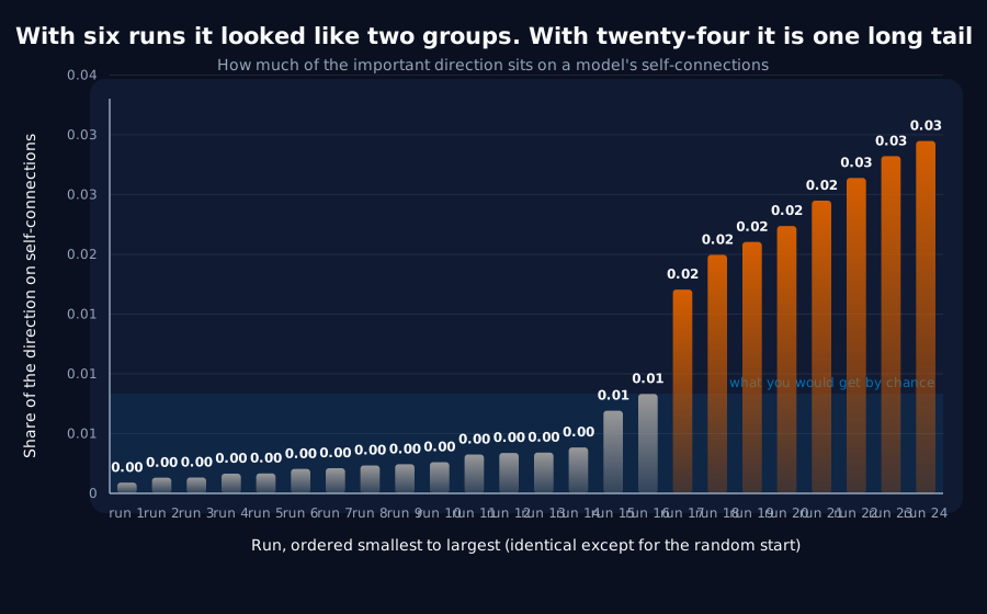
What we found. We ran it six times and got two results, and we have since run it eighteen more times and both of them were wrong. The first six looked like they fell into two clean groups, three high and three low with nothing in between. That gap filled in as soon as we added runs: the real picture is one lopsided spread, most runs low and a few much higher, and the six we happened to start with were on the high side. The second correction goes the other way. With six runs the effect we were testing for did not clear our bar, so we reported the two findings as unrelated. With twenty-four it does clear it, in twenty of the twenty-four. They are related after all, and we had simply not run enough to tell.

Why it matters. Two notes on how we are reporting this. The honest version of the finding needs both halves: against the right yardstick that important direction does lean on the self-connections, but in absolute terms a typical run still puts less weight there than pure chance would. It leans that way less reluctantly than everything else does, which is not the same as leaning on it. And we have left the original write-up intact underneath with a correction attached, rather than quietly editing it, because the before and after is the useful part: six runs produced two confident readings and both of them were wrong.

The rest of this page is the technical record: the design, every number, and the limits. It is written for a reviewer, and you do not need it to have understood the result above.

New here? How to read a research record

Start at the verdict. Every record states, before the experiment was run, what result would have made us abandon the idea. That is the "kill test". Then it says whether the test fired. Nothing gets reinterpreted after the fact.
Numbers in square brackets are uncertainty. 23.4 [18.1, 28.7] means our best estimate is 23.4 and the true value is probably somewhere in that range. If a range includes zero, we cannot claim an effect.
Negative results are kept. Roughly half of what is published here says an idea did not work, including several of our own. Those pages are not failures, they are the output. Work that only publishes what worked is not measuring anything.
Read the Limits section. Every record ends with what it does not show. It is the most honest part of any experiment and usually the shortest.
Pro tip: the figures near the top are designed to carry the result on their own. If you read nothing else, read the caption under each one, which says what it shows and what to take from it.

CORRECTION, 2026-08-24: this record's headline is superseded by its own follow-up. The pilot was re-run with 18 additional seeds (24 in total, the original six kept and marked). Two things changed, in opposite directions, and both are in the update section at the end: - The bimodal split does not survive. Five of the eighteen fresh seeds land inside the gap the first six left empty, and the distribution is a right-skewed continuum rather than two groups. "Half the seeds say yes" was a six-seed artifact, and the original six were unrepresentative: they average 1.66x the uniform share against the fresh eighteen's 1.02x. - The kill test now goes the other way. On 24 seeds the paired difference is +0.0077 [+0.0033, +0.0121], clear of zero, and positive in 20 of 24 runs. The diagonal claim is supported after all, modestly: the leading direction carries 4.6x what its own span-random control does. The text below is the six-seed record as originally written and is left unchanged. Read the update for the current reading.

EXPLORATORY. Not a preregistered study. Local CPU, 12 training runs, no GPU, no cost.

Program v2 Bucket I, item I3. Decisive computation: analysis/direction_anatomy.py. Output: analysis/direction_anatomy.json. Reproduce with python analysis/direction_anatomy.py in about ten minutes on a throttled laptop CPU.

The question

Two results point at the same object from different sides and had never been compared.

**With six runs it looked like two groups. With twenty-four it is one long tail.** Two of our earlier findings pointed at the same part of a model from different directions. One found that a single direction of change carries most of what matters during learning. The other found that a unit's connection to itself, which is how it remembers, explains much of why one way of trimming a model beats another. This asks whether they are the same thing, by measuring how much of that important direction sits on those self-connections. The blue band is what you would get by pure chance. We first ran six of these and saw what looked like two clean groups; this is the same chart after adding eighteen more. The gap filled in. What looked like two separate groups on six runs is one skewed spread on twenty-four, with most runs low and a handful much higher, so we withdrew the two-groups reading. But the extra runs also settled the original question the other way: with enough of them, the important direction does reliably put more weight on self-connections than our comparison does, in twenty of twenty-four runs. Both halves matter, because the six-run version got each of them wrong in a different direction.

F4: a single gradient direction carries 61% of the critical period for 14% of the gradient's energy.

G4: a unit's connection to itself explains 38-50% of the advantage structured sparsity has over random sparsity at matched connection count. The diagonal of the recurrent matrix is how a gated recurrent unit retains state at all.

Are they the same thing? If the load-bearing direction lives on the diagonal, this programme has one mechanism where it reports two.

Kill test: the top direction's mass on the diagonal is no higher than a span-random direction's.

The control is F4's span-random direction, not a uniformly random one: a random orthonormal mixing of the same buffer of recent gradients, so it is gradient-like in every respect except being the leading one. A GRU stacks three gates, so a unit's self-connection is three entries (rows i, i+W, i+2W, each at column i): 144 of 17,280 parameters, a uniform share of 0.83%.

Result: the kill test fires by its letter, and the population splits

Group	Top direction	Span-random control	Uniformly random	Uniform share
recurrent diagonal	`0.0138`	`0.0025`	`0.0086`	`0.0083`
recurrent, off-diagonal	`0.1045`	`0.0695`	`0.3859`	`0.3917`
input to recurrence	`0.4627`	`0.6912`	`0.4052`	`0.4000`
embedding and head	`0.2346`	`0.1736`	`0.1775`	`0.1778`
biases and norm	`0.1844`	`0.0632`	`0.0228`	`0.0222`

Paired within run, top minus span-random on the diagonal: +0.0113 [-0.0005, +0.0231], the interval crosses zero, so by the letter of the kill test the diagonal claim is not supported.

But the interval crosses zero because the seeds split rather than scatter:

Seed	Diagonal mass	Relative to uniform
9007	`0.0024`	`0.29x`
9043	`0.0033`	`0.39x`
9029	`0.0038`	`0.46x`
9041	`0.0224`	`2.68x`
9011	`0.0245`	`2.94x`
9001	`0.0264`	`3.17x`

Three seeds put roughly three times the uniform share on the diagonal; three put less than half. There is no overlap and no middle. That is two behaviours, not one noisy one, and "no effect on average" is the wrong summary of it.

Two things the sweep adds

The enrichment is specific to the leading direction. Diagonal mass by subspace rank:

Rank	Leading subspace	Span-random	Uniform
1	`0.0138`	`0.0025`	`0.0083`
2	`0.0131`	`0.0023`	`0.0083`
4	`0.0085`	`0.0024`	`0.0083`
8	`0.0050`	`0.0026`	`0.0083`

It dilutes steadily as the subspace grows and is at the uniform share by rank 4. Whatever this is, it is a property of the first direction, which is the one F4 showed to be load-bearing.

Gradients as a class avoid the diagonal. The span-random control sits at 0.0025, about 0.3x the uniform share, at every rank. So the leading direction is not merely at the uniform level in the enriched seeds: it is 9x to 10x what a gradient-like direction from the same subspace puts there. The paired difference understates that because it is dominated by the three unenriched seeds.

Verdict

By the letter, the kill test fires. The diagonal claim is not supported on this evidence, and F4's direction and G4's self-connections cannot be reported as one mechanism.
By the intent, the answer is "sometimes", which was not on the menu. The load-bearing direction is strongly diagonal-enriched in half the runs and not at all in the other half, on identical configurations differing only by seed.
What distinguishes the two groups is not measured here, and is the obvious follow-up. It is also the more interesting question than the one this item asked.
The programme still reports two mechanisms rather than one.

Limits

Six seeds, three per group. A 3-3 split on six runs is exactly the sample size at which a bimodal pattern could still be chance. The gap between groups is large (0.0038 against 0.0224, no overlap) but the count is small, and the first thing a follow-up should do is add seeds.
One width, one task, one architecture, one learning rate, one window position.
The direction is taken at one step, the end of F4's projection window. Whether a run's group membership is stable across the window, or flips, is untested and is cheap to check.
This measures where the direction's mass sits, not what it does. A direction could be diagonal-enriched and not causally about self-retention, or causally about it while spread across many parameters. F4's surgery is the causal instrument; this is anatomy.
The paired endpoint was preregistered before the split was visible. The split is reported as an observation about the population, not as a revised endpoint.

Update, 2026-08-24: eighteen more seeds

The record above ends by saying a 3-3 split on six runs is exactly the sample size at which a bimodal pattern could still be chance, and that the first thing a follow-up should do is add seeds. This is that follow-up: 18 fresh seeds, the original six kept and marked, 24 in total. Same configuration, same window, same controls.

The split dissolves

Where the 18 fresh seeds landed	Count
below `0.5x` uniform (the lower group)	11
inside the gap the first six left empty (`0.5x`-`2.6x`)	5
above `2.6x` uniform (the upper group)	2

The middle fills in. Pooled across all 24 runs the distribution is a right-skewed continuum, quartiles 0.11x, 0.25x, 0.41x, 2.52x, 3.54x of the uniform share, with a heavy cluster low and a long upper tail. The largest gap anywhere in the pooled sample is 1.05x wide at 1.52x, which is 31% of the range: a relative sparsity in the middle, not two populations.

And the original six were unrepresentative. They average 1.66x the uniform share; the eighteen fresh seeds average 1.02x. The discovery sample was biased upward, which is what a 3-3 split found by looking should be assumed to be until tested.

"Half the seeds say yes" was a six-seed artifact.

But the kill test now goes the other way

	6 seeds	24 seeds
paired difference, top minus span-random	`+0.0113` `[-0.0005, +0.0231]`	`+0.0077` `[+0.0033, +0.0121]`
clears zero	no	yes
runs with a positive difference	,	20 of 24
leading direction vs its own control	`5.5x`	`4.6x` (`0.0099` against `0.0021`)

With adequate power the diagonal claim is supported. The interval is clear of zero, the effect is positive in 20 of 24 runs with a median of +0.0017, so it is not a tail artifact.

Two things have to be said together, and neither alone is honest:

Against its own control, the leading direction is consistently diagonal-enriched, 4.6x the span-random direction drawn from the same buffer, positive in 20 of 24 runs.
**Against the uniform share, the typical run is still diagonal-*poor***, median 0.41x. The mean of 1.18x is pulled up by the tail. Gradients as a class avoid the diagonal hard (control median 0.22x uniform), and the leading direction avoids it less.

So the leading direction is not concentrated on the diagonal in any absolute sense. It is systematically less averse to it than the rest of the gradient subspace is.

One covariate survives a family-wise test

Five cheap covariates measured on the same buffer, against a family-wise null over all five (20,000 permutations, largest |r| per draw, critical value 0.505):

Covariate	`r` with diagonal mass
buffer norm	`-0.576` (beats the null)
transition step	`-0.503`
top share of spectrum	`-0.377`
spectral gap (`s1/s2`)	`-0.288`
final accuracy	`+0.072`

Runs with smaller gradients at the transition put more of the leading direction on the diagonal. The spectral-gap hypothesis: that a nearly-degenerate top direction would have arbitrary composition, does not survive (-0.288). Buffer norm and transition step are themselves correlated, so this identifies a direction of association, not a cause.

What this changes

I3's answer is now "yes, modestly", not "sometimes". F4's direction and G4's self-connections are related, and the earlier conclusion that they are independent findings was underpowered.
The split reported above is withdrawn as a finding, and stands only as a warning about reading structure into six runs.
The claim to make is the relative one. "The load-bearing direction is enriched on the diagonal relative to gradient-like directions from the same subspace" is supported. "The load-bearing direction lives on the diagonal" is not: the typical run puts less than the uniform share there.
Limits carried forward: still one width, one task, one architecture, one learning rate, one window position, and still anatomy rather than causation, F4's surgery is the causal instrument.

Terms on this page

Every piece of vocabulary this record uses, in plain language. Generated from the text above, so it cannot drift out of step with it.

accuracy: The fraction of answers a model gets right on questions it was not trained on.
architecture: The blueprint of a model: what components it has and how they connect. Two models can be the same size and completely different architectures.
critical period: A stretch of time during which something has to happen for development to proceed normally. Borrowed from biology, where it describes windows in which a young brain must receive certain input.
gated: A design where the model has explicit internal switches deciding what to remember and what to discard at each step. GRUs and LSTMs are gated; plain recurrent networks are not.
gradient: The direction and amount by which each of a model's internal numbers should change to do slightly better. Training is repeatedly following it.
GRU: Gated Recurrent Unit. A compact design for processing sequences one item at a time, with internal switches controlling what it keeps in memory.
kill test: A condition written down before running the experiment that says what result would make us abandon the idea. Fixing it in advance is what stops a disappointing result being reinterpreted as an encouraging one.
learning rate: How big a step training takes each time it updates the model. Too small and nothing happens; too big and it never settles.
parameters: The adjustable numbers inside a model. Training is the process of setting them. Model size is usually quoted as a count of these.
rank: How many independent directions a set of numbers really uses. A low-rank structure is one that looks high-dimensional but is actually simple underneath.
recurrent: A design that reads a sequence one item at a time, carrying memory forward. The main alternative is attention, which looks at everything at once.
seed: The number that fixes all the randomness in a training run. Same seed, same run. Running several seeds is how you tell a real effect from a lucky one.
subspace: A slice of a model's internal space: some directions kept, the rest ignored.
width: How many internal numbers a model uses at each layer. The usual way we vary model size in these experiments.

About this record. This page is the write-up of an experiment we ran ourselves. Every number on it comes from a run we recorded, and the script that produced each one is named in the text above. We publish these results and the data behind them here, including the ones that went against what we expected.

Why we do this. The same care shown above is what we apply to client work. We build custom AI models that you own and run yourself, using our own platform, and the reason we publish research like this is that a model is only worth what its evaluation is worth. If a supplier cannot show you the experiments that went against them, you cannot check the ones that went their way.

All research from this programme →