How do you know a fine-tuned AI model is actually better?

You measure it. Hold out a portion of the client's real examples so the model never sees them during training, score the plain base model on those held-out questions first, fine-tune, then score again on the identical questions with identical scoring. The difference is the lift. Because the only thing that changed is the fine-tune, the improvement is attributable to it.

Does fine-tuning actually improve accuracy, or is the base model already good enough?

It depends on the task and, critically, on how much data you have. On a public benchmark of 510 lawyer-annotated commercial contracts, a base Qwen3-4B extracted short contract fields at 62.2% accuracy. Fine-tuned on 396 examples it reached 83.5-85.4%, a lift of 21.3 to 23.2 points across three runs. The same model trained on only 48 examples produced a lift inside the noise floor, so the amount of data was the deciding factor rather than the model's ceiling.

How much of our own data do we need to fine-tune a model?

Fewer examples than most people expect, but more than a handful. In our contract-extraction measurements, 48 training examples produced no measurable improvement while roughly 400 produced a 22-point gain. The honest answer for any specific case is that it depends on how varied and how consistent the examples are, which is what a paid readiness assessment measures on the client's own corpus.

Why can't you just use a public AI benchmark score?

Public benchmarks measure general ability on standardised tests, not your work. A model that scores well in the abstract can still be mediocre at reading your contracts or following your policies. Public benchmarks are also increasingly targeted during training, so a high score can reflect test preparation as much as capability. The only benchmark that answers your question is built from your own tasks.

Research record 28 of 39

The Method That Looked Fastest Was Cheating

By Joshua Bolick, Awareness Software Group ~9 min read August 2026

Ongoing research. This is an experimental result from active work, not a settled conclusion. The numbers are what we measured and the method is described so you can judge it, but the programme is still running and later experiments may revise what it means. More about this programme.

In plain English

What we asked. If you are training a model and could choose which examples to train on, the appealing idea is to pick the ones it has most to learn from. We tested several ways of doing that on a task with an easy half and a hard half, against the baseline of simply taking whatever arrives.

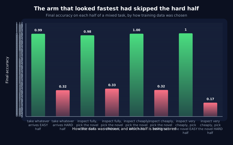
What we found. None of them helped, including one given perfect information at a cost no real system could afford. But one method appeared to: it reached the finish line 26 steps sooner than everything else. It did that by training almost entirely on the easy half, choosing the hard half 9% of the time against the baseline's 51%. It finished perfect on the easy half and worse than the baseline on the hard one.

Why it matters. Our own measurement is what let that pass. We were timing when each model crossed the midpoint of its own progress, and a model that learns half a task has less progress to make, so it crosses its own midpoint sooner and looks fast. The fix is obvious once seen: check what each model actually learned before crediting it with being quick. The broader point is that a cheap shortcut for choosing data will tend to find the easy data, because easy and informative look similar to a simple measure and are not the same thing.

The rest of this page is the technical record: the design, every number, and the limits. It is written for a reviewer, and you do not need it to have understood the result above.

New here? How to read a research record

Start at the verdict. Every record states, before the experiment was run, what result would have made us abandon the idea. That is the "kill test". Then it says whether the test fired. Nothing gets reinterpreted after the fact.
Numbers in square brackets are uncertainty. 23.4 [18.1, 28.7] means our best estimate is 23.4 and the true value is probably somewhere in that range. If a range includes zero, we cannot claim an effect.
Negative results are kept. Roughly half of what is published here says an idea did not work, including several of our own. Those pages are not failures, they are the output. Work that only publishes what worked is not measuring anything.
Read the Limits section. Every record ends with what it does not show. It is the most honest part of any experiment and usually the shortest.
Pro tip: the figures near the top are designed to carry the result on their own. If you read nothing else, read the caption under each one, which says what it shows and what to take from it.

EXPLORATORY. Not a preregistered study. Local CPU, 20 training runs, no GPU, no cost.

Program v2 Bucket G, item G5. Decisive computation: analysis/heterogeneous_novelty.py. Output: analysis/heterogeneous_novelty.json. Reproduce with python analysis/heterogeneous_novelty.py in about thirty-five minutes on a throttled laptop CPU.

The question

B4 found no benefit to gradient-novelty data selection, every arm indistinguishable from taking the first batch that arrived, including a full-gradient arm with perfect information at impractical cost, which saved +0.4 steps out of 93.6.

**The arm that looked fastest had skipped the hard half.** Training data was drawn from two versions of the same task, one easy and one hard, and each method chose which batch to train on. Green bars are final accuracy on the easy half, pink on the hard half. The leftmost pair is the control, which just takes whatever arrives. The rightmost method reached the moment of learning about 26 steps sooner than the control, which on a speed chart looks like the one approach that works. It got there by training almost entirely on the easy half: it chose the hard half 9% of the time against the control's 51%, ended perfect on the easy half, and ended WORSE than the control on the hard one. It was not finding informative data, it was avoiding difficult data. We only caught it because speed was measured against how much each model actually learned, and a model that learns half a task reaches the middle of its own smaller range sooner.

B4 named its own most likely explanation in Limits: its batches are drawn i.i.d. from one distribution, so there may be genuinely nothing to select between. Until that is tested, B4 cannot be cited as a result about the method rather than about that task.

Kill test: selection is still indistinguishable from random on heterogeneous data. Then novelty selection does not work as a method, and the line closes rather than being scoped.

The mixture

Each candidate batch comes from one of two sub-tasks chosen at random: delayed-copy at lag 2 and at lag 8. Same vocabulary, same length, same scoring, genuinely different structure. Everything else is B4 unchanged, so a difference must be the data rather than the design.

Result: the kill test fires

Arm	Transition	Final easy / hard	Harder half chosen	Beats control?
random (control)	`91.6` `[76.8, 106.4]`	`0.994` / `0.316`	51.4%	,
full gradient	`97.2` `[75.8, 118.6]`	`0.976` / `0.335`	68.2%	no
head, closed form	`97.6` `[78.3, 116.9]`	`0.995` / `0.319`	61.0%	no
embedding	`65.6` `[58.7, 72.5]`	`1.000` / `0.166`	8.7%	see below

The full-gradient arm still does not beat random, on data that genuinely varies, with perfect information about every candidate. That is B4's result reproduced in the regime B4 said might explain it away. B4's null is about the method, not about its task.

The arm that appeared to win

The embedding arm "saves" 26 steps with an interval clear of the control's. On the summary that reads as the one selector that works.

It is not selecting informative data. It is avoiding difficult data.

It chose the harder sub-task 8.7% of the time against the control's 51.4%, a -42.8% skew.
It reached 1.000 on the easy sub-task and 0.166 on the hard one, against the control's 0.316. It is worse than random at the half it avoided.
Its mean accuracy is 0.583 against the control's 0.655.

It trained almost exclusively on the easy half, perfected it, and got worse than chance-adjacent at the other.

Why the measurement let that pass

A transition is defined on each run's own accuracy range. A model that learns only half the mixture has a smaller range, so its midpoint arrives earlier, it looks faster while learning strictly less. Speed was being measured without checking what got learned, and a selector that skips the hard sub-task produces exactly that signature.

The fix is not subtle: record final accuracy per sub-task, and refuse to credit a saving from an arm that has not reached the control's accuracy. A speed comparison between models that learned different amounts is not a speed comparison.

The first run's verdict called this "found a curriculum rather than novelty selection", which was too generous. A curriculum is easy-then-hard. This is easy-and-never-hard.

Verdict

B4's null stands and is now about the method. On genuinely heterogeneous data, the full-gradient arm, the upper bound on what any selector could know, is still indistinguishable from taking whatever arrives.
No arm both beats the control and learns as much.
The one arm that looked like a win was avoiding the hard half, and would have been published as a success by any summary that reported speed without accuracy.
Gradient-novelty data selection is closed, on i.i.d. data by B4 and on mixed data by G5.

Limits

Two sub-tasks, one width, one optimizer, five seeds, 460 steps.
The hard sub-task is not solved by anyone. All arms end between 0.166 and 0.335 on lag 8, so this measures selection during partial learning of the hard half rather than through its completion. A longer budget would test whether selection matters when both halves are learnable, and is the obvious follow-up.
The mixture is 50/50 and uniform. A skewed or shifting mixture is a different experiment, and arguably the one closest to real training data.
The embedding arm's behaviour is itself a finding about proxies, not just an artifact to discard: the cheapest signal available correlated almost perfectly with sub-task identity, so it became a difficulty detector. A cheap proxy that tracks difficulty rather than informativeness is a predictable failure mode for any selection scheme built on one.
Accuracy tolerance for crediting a saving is 0.02, chosen before the comparison rather than after.

Terms on this page

Every piece of vocabulary this record uses, in plain language. Generated from the text above, so it cannot drift out of step with it.

accuracy: The fraction of answers a model gets right on questions it was not trained on.
gradient: The direction and amount by which each of a model's internal numbers should change to do slightly better. Training is repeatedly following it.
kill test: A condition written down before running the experiment that says what result would make us abandon the idea. Fixing it in advance is what stops a disappointing result being reinterpreted as an encouraging one.
optimizer: The algorithm that decides how to change the model given the gradient. AdamW and SGD are two common choices and they behave differently.
seed: The number that fixes all the randomness in a training run. Same seed, same run. Running several seeds is how you tell a real effect from a lucky one.
vocabulary: The set of distinct symbols a model can read and produce.
width: How many internal numbers a model uses at each layer. The usual way we vary model size in these experiments.

About this record. This page is the write-up of an experiment we ran ourselves. Every number on it comes from a run we recorded, and the script that produced each one is named in the text above. We publish these results and the data behind them here, including the ones that went against what we expected.

Why we do this. The same care shown above is what we apply to client work. We build custom AI models that you own and run yourself, using our own platform, and the reason we publish research like this is that a model is only worth what its evaluation is worth. If a supplier cannot show you the experiments that went against them, you cannot check the ones that went their way.

All research from this programme →