How do you know a fine-tuned AI model is actually better?

You measure it. Hold out a portion of the client's real examples so the model never sees them during training, score the plain base model on those held-out questions first, fine-tune, then score again on the identical questions with identical scoring. The difference is the lift. Because the only thing that changed is the fine-tune, the improvement is attributable to it.

Does fine-tuning actually improve accuracy, or is the base model already good enough?

It depends on the task and, critically, on how much data you have. On a public benchmark of 510 lawyer-annotated commercial contracts, a base Qwen3-4B extracted short contract fields at 62.2% accuracy. Fine-tuned on 396 examples it reached 83.5-85.4%, a lift of 21.3 to 23.2 points across three runs. The same model trained on only 48 examples produced a lift inside the noise floor, so the amount of data was the deciding factor rather than the model's ceiling.

How much of our own data do we need to fine-tune a model?

Fewer examples than most people expect, but more than a handful. In our contract-extraction measurements, 48 training examples produced no measurable improvement while roughly 400 produced a 22-point gain. The honest answer for any specific case is that it depends on how varied and how consistent the examples are, which is what a paid readiness assessment measures on the client's own corpus.

Why can't you just use a public AI benchmark score?

Public benchmarks measure general ability on standardised tests, not your work. A model that scores well in the abstract can still be mediocre at reading your contracts or following your policies. Public benchmarks are also increasingly targeted during training, so a high score can reflect test preparation as much as capability. The only benchmark that answers your question is built from your own tasks.

Research record

The Shortcut Reversed

By Joshua Bolick, Awareness Software Group ~13 min read September 2026

Ongoing research. This is an experimental result from active work, not a settled conclusion. The numbers are what we measured and the method is described so you can judge it, but the programme is still running and later experiments may revise what it means. More about this programme.

Part of a bigger question: How do we know our own results are real? – Repeatedly, the control rather than the measurement decided the result -- and several striking findings dissolved when the right comparison was finally run.

In plain English

What we asked. Training a model is expensive, so a shortcut that reaches the same quality on less data is worth real money. We had found one: partway through training, switch to a cheaper setting that processes a quarter as much data per step. On our smaller models that reached the target on 22% less data. The catch was that switching at a completely random moment worked just as well, so the early-warning signal we had built to tell us when to switch was contributing nothing, and detecting it cost more than the shortcut saved.

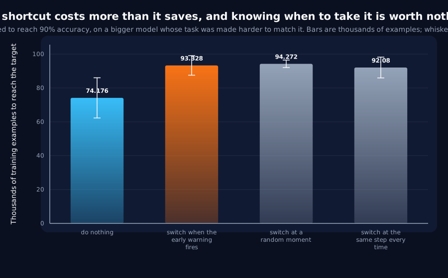
What we found. That result was measured on one model size, and we have since learned that measuring something at one size while holding the task fixed makes the model progressively oversized and can invent effects that are not there. So we repeated it on a model four times wider, with the task made harder to match. The shortcut has reversed: it now needs about a quarter more data than simply not taking it, and the gap is larger than our measurement uncertainty. And the timing is still worth nothing, now with twice as much warning: switching when the warning fires, at a random moment, or at the same fixed step in every run all land in the same place.

Why it matters. The most useful part is a correction to our own accounting. We had priced the early-warning instrument at 55% of the training budget, which sounded bad enough. That figure counted rows of data, and it turns out rows of data cancel out of the ratio entirely, so the number could not respond to model size at all. Priced in the arithmetic actually performed, the instrument cost nearly twice the whole training budget at the smaller size and 27% at the larger one. So the instrument really does become far more affordable as models grow, roughly sevenfold. It is just that the thing it was buying went negative at the same time. A cost ratio has to be measured in units that can respond to whatever you are varying, or it will quietly answer a different question.

The rest of this page is the technical record: the design, every number, and the limits. It is written for a reviewer, and you do not need it to have understood the result above.

New here? How to read a research record

Start at the verdict. Every record states, before the experiment was run, what result would have made us abandon the idea. That is the "kill test". Then it says whether the test fired. Nothing gets reinterpreted after the fact.
Numbers in square brackets are uncertainty. 23.4 [18.1, 28.7] means our best estimate is 23.4 and the true value is probably somewhere in that range. If a range includes zero, we cannot claim an effect.
Negative results are kept. Roughly half of what is published here says an idea did not work, including several of our own. Those pages are not failures, they are the output. Work that only publishes what worked is not measuring anything.
Read the Limits section. Every record ends with what it does not show. It is the most honest part of any experiment and usually the shortest.
Pro tip: the figures near the top are designed to carry the result on their own. If you read nothing else, read the caption under each one, which says what it shows and what to take from it.

EXPLORATORY. Not a preregistered study. Local CPU, 44 training runs, no GPU, no cost.

Program v2 Bucket Q, item Q1. Decisive computation: analysis/spend_the_lead_matched.py. Output: analysis/spend_the_lead_matched.json. Reproduce with python analysis/spend_the_lead_matched.py; --reuse re-derives every endpoint without retraining.

The question

J7 is the result everything efficiency-shaped in this programme defers to. At the decode probe's crossing it cut the batch by 4x and found three things: no accuracy gain at a matched sample budget; a real 22% saving in samples-to-target that a random-timed switch matched exactly; and an instrument costing 55.4% of the training budget to find a moment worth 2,460 samples.

**The shortcut costs more than it saves, and knowing when to take it is worth nothing.** An earlier experiment found that switching to a cheaper training setting partway through reached the target on 22% less data, but that switching at a random moment worked just as well, so the early warning that told us when to switch was worth nothing. This repeats it on a model four times wider, with the task made harder so the model is not simply oversized. Two things changed and neither helps. The shortcut itself has reversed: it now needs about a quarter more data than not taking it, and the difference is larger than the measurement uncertainty. And the timing is still worth nothing, at twice the warning we had before: switching when the warning fires, at a random moment, or at the same fixed step every run all land in the same place. A shortcut that worked at one model size can reverse at another, which is a reason to re-check the shortcut and not only the instrument.

It was measured at width 48 on the fixed task, which is the condition P11 and P12 showed was confounded for six other results. Both halves were in question, and for opposite reasons: on a matched ladder the same probe's lead grows with width (14.8 steps at 32 to 39.9 at 192), and a cost expressed as a ratio has a denominator that grows with width while its numerator may not.

Kill test, fixed before execution: at matched difficulty and width 192 the probe-timed arm still fails to beat a random-time-matched arm at equal sample budget, and the probe's cost remains above the saving it produces. Both must fail for J7's conclusion to stand as written.

The anchor reproduces J7 exactly

J7's configuration re-run here: width 48, lag 4, J7's eight seeds, J7's 57,600-sample budget, through the same probe:

Arm	Samples to 0.9, here	J7 published
control	`11,080` `[10,380, 11,780]`	`11,080` `[10,380, 11,780]`
probe-timed	`8,620` `[7,976, 9,264]`	`8,620` `[7,976, 9,264]`
random-timed	`8,610` `[7,951, 9,269]`	`8,690` `[8,148, 9,232]`

Identical for the two deterministic arms; the random arm differs because this pilot seeds its draw per run, and the intervals overlap. Row overhead reproduces at 55.4%. The precondition is enforced in code and no verdict prints without it.

Result: the kill test fires, and the manoeuvre has reversed sign

Width 192, lag 11 (P12's matched ladder), five seeds, 192,000 samples per arm, 3,000 control steps. The probe crossed in all five runs, at steps 140 to 200.

Arm	Final accuracy	Samples to 0.9	Switch
control	`0.9827` `[0.9693, 0.9961]`	`74,176` `[62,290, 86,062]`	,
probe-timed	`0.9674` `[0.9538, 0.9810]`	`93,328` `[87,561, 99,095]`	`165`
random-timed	`0.9706` `[0.9637, 0.9775]`	`94,272` `[92,054, 96,490]`	`173`
fixed-schedule	`0.9688` `[0.9629, 0.9746]`	`92,080` `[85,936, 98,224]`	`165`

The batch cut costs 25.8% more samples instead of saving 22%, and the probe-timed and control intervals do not overlap, so the cost is real rather than noise. J7's one positive observation: that cutting the batch genuinely works, does not transfer to the matched ladder.

The timing still buys nothing, at twice the lead. Probe-timed 93,328, random-timed 94,272, one fixed step for every seed 92,080. Every interval overlaps every other, and the arm with no information at all is nominally the best of the three. This is J7's central finding, confirmed where the probe's warning is about twice as long.

The cost half moved exactly as predicted, and it corrects J7's own number

The instrument was priced two ways: J7's unit, scored rows, and the arithmetic it actually performs.

Block	Overhead in rows	Overhead in arithmetic	One probe fit, in training steps
anchor (width 48)	`55.4%`	`188.4%`	`118.0`
matched (width 192)	`43.5%`	`27.3%`	`24.1`

The probe does get much cheaper relative to training as the model grows, 6.9x cheaper in arithmetic, and one fit falls from 118 training steps to 24.1. That was Q1's prediction and it holds.

But J7 understated its own instrument by 3.4x. In arithmetic the probe cost nearly twice the entire training budget at width 48, not 55.4% of it. J7's conclusion is unaffected: it was already an order of magnitude the wrong way, but the number in its record is a floor, not the cost.

Why the row unit could not have answered this

overhead_rows counts scored rows in both numerator and denominator, so the scored-positions factor cancels and it reduces to

`` crossing_step PROBE_BATCH / (EVAL_EVERY budget_samples) ``

Width does not appear. Every change from 55.4% to 43.5% is the longer budget; none of it is the width. A training row at width 192 costs about 15x a training row at width 48, while a probe row costs about 3x, and a unit that cancels that difference cannot see it.

A cost ratio has to be denominated in a unit that responds to the axis under test. This is the same shape of error as Q6's: a quantity divided by the wrong thing answers a question nobody asked.

Verdict

The kill test fires. J7's negative survives, and more firmly than before: at matched difficulty the manoeuvre does not merely fail to beat random timing, it costs a quarter more samples than not doing it.
The two halves moved in opposite directions. The instrument got 6.9x cheaper relative to training; the thing it was buying went negative. An instrument becoming affordable is not the same as its output becoming worth buying.
J7's record gains a correction banner for the arithmetic cost, not for its conclusion.
An efficiency manoeuvre validated at one width can reverse sign at another. P11 and P12 restored instruments across width; nobody had re-checked a manoeuvre. This is the first one re-checked and it reversed.

Limits

Five seeds in the matched block against J7's eight, because each switched arm runs 11,500 steps at 16x the arithmetic per step. Intervals are correspondingly wide, and the control's is the widest of the four.
The random-time-matched arm draws from five observed crossings, so coincidences happen: on seed 5101 it drew 175, the probe's own answer, making that pair of runs identical. That is correct behaviour for a distribution-matched control and it narrows the comparison.
Why the cut hurts here is not established. A plausible reading is that lag 11 leaves five scored positions per sequence, so a batch of 16 carries 80 scored tokens against 320, and the harder task needs more signal per step. That is speculation; nothing here tests it.
The arithmetic model is a model. It counts multiply-accumulates in the GRU's gates and head and takes backward as twice forward. It is written out in the committed script and is deliberately not a wall-clock measurement, which under a duty-cycle throttle on tiny models measures framework overhead more than arithmetic.
One manoeuvre, one probe configuration, one task family. The 4x batch cut and the 0.5 crossing were fixed in advance by J7 and neither was swept.
Final accuracy differences between arms are inside overlapping intervals and nothing is claimed from them; samples-to-target carries the result, as it did in J7.

Terms on this page

Every piece of vocabulary this record uses, in plain language. Generated from the text above, so it cannot drift out of step with it.

accuracy: The fraction of answers a model gets right on questions it was not trained on.
GRU: Gated Recurrent Unit. A compact design for processing sequences one item at a time, with internal switches controlling what it keeps in memory.
kill test: A condition written down before running the experiment that says what result would make us abandon the idea. Fixing it in advance is what stops a disappointing result being reinterpreted as an encouraging one.
probe: A small separate model trained to read information out of a bigger model's internals, used as a measuring instrument rather than as a product.
seed: The number that fixes all the randomness in a training run. Same seed, same run. Running several seeds is how you tell a real effect from a lucky one.
width: How many internal numbers a model uses at each layer. The usual way we vary model size in these experiments.