How do you know a fine-tuned AI model is actually better?

You measure it. Hold out a portion of the client's real examples so the model never sees them during training, score the plain base model on those held-out questions first, fine-tune, then score again on the identical questions with identical scoring. The difference is the lift. Because the only thing that changed is the fine-tune, the improvement is attributable to it.

Does fine-tuning actually improve accuracy, or is the base model already good enough?

It depends on the task and, critically, on how much data you have. On a public benchmark of 510 lawyer-annotated commercial contracts, a base Qwen3-4B extracted short contract fields at 62.2% accuracy. Fine-tuned on 396 examples it reached 83.5-85.4%, a lift of 21.3 to 23.2 points across three runs. The same model trained on only 48 examples produced a lift inside the noise floor, so the amount of data was the deciding factor rather than the model's ceiling.

How much of our own data do we need to fine-tune a model?

Fewer examples than most people expect, but more than a handful. In our contract-extraction measurements, 48 training examples produced no measurable improvement while roughly 400 produced a 22-point gain. The honest answer for any specific case is that it depends on how varied and how consistent the examples are, which is what a paid readiness assessment measures on the client's own corpus.

Why can't you just use a public AI benchmark score?

Public benchmarks measure general ability on standardised tests, not your work. A model that scores well in the abstract can still be mediocre at reading your contracts or following your policies. Public benchmarks are also increasingly targeted during training, so a high score can reflect test preparation as much as capability. The only benchmark that answers your question is built from your own tasks.

Research record

Latent Knowledge Before Behaviour

By Joshua Bolick, Awareness Software Group ~7 min read August 2026

Ongoing research. This is an experimental result from active work, not a settled conclusion. The numbers are what we measured and the method is described so you can judge it, but the programme is still running and later experiments may revise what it means. More about this programme.

EXPLORATORY. Not a preregistered study. Local CPU, 10 training runs, no GPU, no cost.

Program v2 tier 2, item F2. Decisive computation: analysis/decode_probe.py. Output: analysis/decode_probe.json. Reproduce with python analysis/decode_probe.py in about twelve minutes on a throttled laptop CPU.

The question

Every signal this program has found is coincident with the transition, or worse. The geometry peak lands at the transition under AdamW and 243 steps after it under SGD (D8). No early-trajectory metric ranks final outcomes (K1). Every controller idea in Bucket C needs something that arrives first, and nothing did.

**The answer is readable before the model can say it.** Two ways of asking what a model knows, measured at every step of training. The lower line is how often it gets the answer right. The upper line is how often the answer can be recovered from its internal state by a readout of exactly the same kind the model itself uses, fitted as well as possible. The dashed line is the same procedure applied to scrambled labels, which should and does stay at chance. The upper line reaches any given level well before the lower one: about 23 steps earlier at the halfway mark, and earlier at every level tested. The information arrives in the model before the model can use it, so the gap between these two lines is an early warning of learning that is about to happen. It is the first such signal this project has found, and an earlier version of the same experiment missed it entirely because the readout was too weak to be trusted.

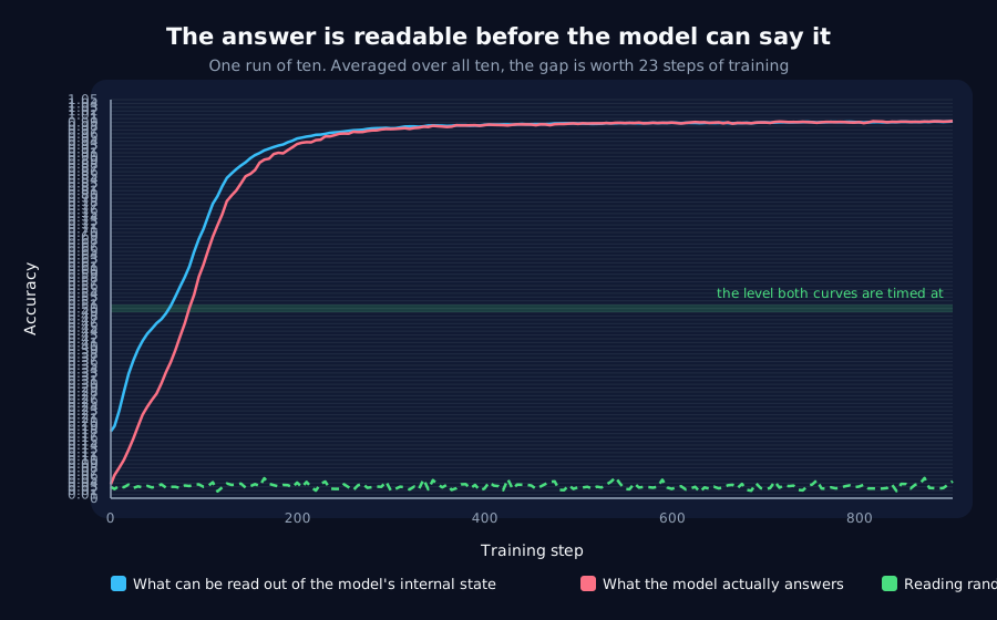
F2 looks in a different place. At each point in training, fit a linear probe from the model's hidden state to the token it is supposed to emit, and compare that probe's accuracy against the model's own.

The probe is the same function class as the output head, a linear map from final_norm to the vocabulary. So this is not asking whether some clever decoder can extract the answer. It asks whether an optimally fitted version of the readout the model already has would beat the one it has learned. If yes, the information is present and the head has not yet learned to read it.

Kill test: decodability and behavioural accuracy rise simultaneously within measurement resolution across ten seeds.

Result: the kill test fails, decisively

Quantity	Value
Probe reaches 50% at step	59.3
Model reaches 50% at step	82.7
Lead	+23.5 steps `[+22.1, +24.9]`
Runs with a lead above the 5-step resolution	10 / 10
Largest probe-minus-model gap	`+0.2071` `[+0.1975, +0.2167]` at step 28

The information is linearly present in the hidden state roughly 23 steps before the model can act on it, on a transition that lands around step 83. That is about 28% of the way to the event, and it is the first genuinely leading signal in this program.

It is not an artifact of the threshold

The 50% crossing was chosen before looking. The lead survives every level tested, and is positive in all ten runs at every one:

Crossing level	Lead (steps)	SD
20%	`+24.6`	1.9
30%	`+35.6`	3.1
40%	`+39.2`	3.8
50%	`+23.5`	1.9
60%	`+14.9`	0.7
70%	`+13.4`	0.9
80%	`+13.6`	1.7
90%	`+17.5`	3.3

The controls hold

Shuffled-label control: 0.0315, against a chance level of 0.0312. A probe of this capacity extracts nothing from noise, so the measured decodability is not fitting artefact.
Instrument check: the probe matches the model at the end in 10 of 10 runs (0.9923 against 0.9917). This is the load-bearing control, for the reason below.

The correction that changes everything about this record

The first version of this pilot returned the opposite verdict, and it was wrong.

	First version	Corrected
Lead	`+1.5` steps `[-0.0, +3.0]`	`+23.5` steps `[+22.1, +24.9]`
Runs with a resolvable lead	1 / 10	10 / 10
Verdict	killed	leading indicator

Nothing about the models changed. The entire verdict flipped on probe strength, through two independent weaknesses:

The probe was the wrong estimator. Closed-form ridge regression onto one-hot targets is a weak classifier at high accuracy. It ended training at 0.9303 while the model reached 0.9917: an optimally fitted readout losing to a trained one by 6 points, which is not possible if the probe is doing its job. It was replaced with a cross-entropy-fitted linear classifier, using the ridge solution as its starting point.
The probe was sample-limited. With 512 sequences it fits 1,568 parameters on 3,328 rows and under-fits badly. Raising the fitting set to ~26,000 scored positions closed the remaining gap.

Crucially, the weakness biased the answer toward the null. The under-powered probe was overtaken by the model before the 50% crossing, so its crossing was delayed by its own incapacity, and the measured lead collapsed toward zero. A weak instrument does not produce noise here; it produces a confident, wrong negative.

Standing rule adopted from this. A null result from a probe is a statement about the probe until the probe is validated against a known-achievable target. Every probe in this project must now clear an instrument check, for a readout probe, matching the trained readout at convergence , and that check must be reported alongside the result.

This is the second time in program v2 that a measurement, not a model, produced the headline: D6 found that the post-peak fall was a property of the measuring frame. Both were caught by asking what the instrument could and could not do, rather than by re-examining the data.

An observation worth carrying to F3

At step 1, before any meaningful training, the probe already reads 0.1761 against the model's 0.0368, about 5.6x chance. A substantial part of the answer is linearly present in an almost untrained recurrent state.

That is the echo-state hypothesis (F3) appearing unbidden: random recurrent dynamics already carry usable information about the lagged token, and part of what training does is learn to read what was largely already there rather than to create it. F3 should be run next, and this pilot has already given it a nonzero prior.

What this changes for the program

The central obstacle is partially removed. Program v2's constraint table records that the transition signal is coincident, not leading. That remains true of the geometry signal. It is now false in general: a decode-probe gap leads by 23 steps.
Bucket C's gate is half-satisfied. The gate requires D3 answering "smooth" and one of F2 / F1 / E4 producing a usable timing signal. F2 has produced one, so D3 is now the sole remaining gate and its priority rises accordingly.
The signal is usable online. The probe needs labels, and during training the labels are in hand. Fitting it is one linear solve plus a short refinement, negligible against a training step.
A4's non-oracle version becomes possible. The transition kick needed to act before the transition and had no way to know when that was. It now has a candidate.

Limits

One architecture (tiny-gru), one task, one width (48), one optimizer (AdamW). D8 showed that timing claims in this project can belong to the optimizer rather than to learning, so F2 under SGD is a required follow-up before anything is built on it.
The lead is measured between two accuracy curves crossing a level. It is not yet demonstrated that the gap predicts the transition step across seeds, with transitions spanning only ~10 steps here there is little variance to correlate against, the same limitation that made A9 unanswerable. Establishing predictive power needs the wider transition spread that a learning-rate or width sweep would give.
23 steps is a real lead but a short one. Whether it is enough to act on is A4's question, not this one.

The plain-language version. This page is the record: the design, the numbers and the limits. If you would rather have the story, Latent Knowledge Before Behaviour, explained without the jargon, covers the same result for a reader who has never seen a training curve.

About this record. This page is the write-up of an experiment we ran ourselves. Every number on it comes from a run we recorded, and the script that produced each one is named in the text above. We publish these results and the data behind them here, including the ones that went against what we expected.

All research from this programme →