How do you know a fine-tuned AI model is actually better?

You measure it. Hold out a portion of the client's real examples so the model never sees them during training, score the plain base model on those held-out questions first, fine-tune, then score again on the identical questions with identical scoring. The difference is the lift. Because the only thing that changed is the fine-tune, the improvement is attributable to it.

Does fine-tuning actually improve accuracy, or is the base model already good enough?

It depends on the task and, critically, on how much data you have. On a public benchmark of 510 lawyer-annotated commercial contracts, a base Qwen3-4B extracted short contract fields at 62.2% accuracy. Fine-tuned on 396 examples it reached 83.5-85.4%, a lift of 21.3 to 23.2 points across three runs. The same model trained on only 48 examples produced a lift inside the noise floor, so the amount of data was the deciding factor rather than the model's ceiling.

How much of our own data do we need to fine-tune a model?

Fewer examples than most people expect, but more than a handful. In our contract-extraction measurements, 48 training examples produced no measurable improvement while roughly 400 produced a 22-point gain. The honest answer for any specific case is that it depends on how varied and how consistent the examples are, which is what a paid readiness assessment measures on the client's own corpus.

Why can't you just use a public AI benchmark score?

Public benchmarks measure general ability on standardised tests, not your work. A model that scores well in the abstract can still be mediocre at reading your contracts or following your policies. Public benchmarks are also increasingly targeted during training, so a high score can reflect test preparation as much as capability. The only benchmark that answers your question is built from your own tasks.

Research record 55 of 67

Looking In The Right Place First

By Joshua Bolick, Awareness Software Group ~14 min read August 2026

Ongoing research. This is an experimental result from active work, not a settled conclusion. The numbers are what we measured and the method is described so you can judge it, but the programme is still running and later experiments may revise what it means. More about this programme.

In plain English

What we asked. You can find out what a prediction depends on by changing one earlier word and seeing how much worse the prediction gets. Do that for every position and you get a picture of where the model is looking. In our task the answer is always a specific earlier word, so there is a right place to look, which is rare enough to be worth using.

What we found. Before any training the model depends on nothing at all. Within about twenty rounds it already depends most on the position that holds the answer, and it does that roughly eighty rounds before it starts getting answers right. That is by far the earliest warning we have found that a model is about to improve, more than three times longer than anything else in this project. It also comes from a comparison rather than a cut-off: we are asking which position matters most, not whether some number crossed a line we chose. That matters, because a line you choose yourself can create the effect you were looking for, and this one cannot.

Why it matters. The unexpected part comes later. A model that has fully solved the task also depends heavily on positions that carry no information about the answer at all -- about half of its total dependence sits on words it does not need. It is tracking the whole repeating pattern rather than simply fetching the right word, which is the same thing our baseline result found from the other direction: a rule that does simply fetch the right word beats the network outright. If you take one practical thing from this page, it is that a model getting the right answers tells you very little about what it is relying on to get them.

The rest of this page is the technical record: the design, every number, and the limits. It is written for a reviewer, and you do not need it to have understood the result above.

New here? How to read a research record

Start at the verdict. Every record states, before the experiment was run, what result would have made us abandon the idea. That is the "kill test". Then it says whether the test fired. Nothing gets reinterpreted after the fact.
Numbers in square brackets are uncertainty. 23.4 [18.1, 28.7] means our best estimate is 23.4 and the true value is probably somewhere in that range. If a range includes zero, we cannot claim an effect.
Negative results are kept. Roughly half of what is published here says an idea did not work, including several of our own. Those pages are not failures, they are the output. Work that only publishes what worked is not measuring anything.
Read the Limits section. Every record ends with what it does not show. It is the most honest part of any experiment and usually the shortest.
Pro tip: the figures near the top are designed to carry the result on their own. If you read nothing else, read the caption under each one, which says what it shows and what to take from it.

EXPLORATORY. Not a preregistered study. Local CPU, 6 training runs, no GPU, no cost.

Program v2 Bucket M, item M3. Decisive computation: analysis/effective_context.py. Output: analysis/effective_context.json. Reproduce with python analysis/effective_context.py, or re-derive every endpoint with --reuse.

The question

Katz's backoff answers "how much context is available" by falling back to less of it when the long context has not been seen. A network has an effective context too, and fifty-five records about the moment a model's behaviour changes had never measured it.

**Which earlier word the prediction actually depends on, as training proceeds.** To find out what a prediction depends on, change one earlier word and see how much worse the prediction gets. Darker means the prediction got much worse, so that position mattered more. In this task the answer is always the word 3 places back, and because the sequence repeats every 4 words, the word 7 places back is the same word again. Those two columns are the right answer; the rest are not. Before any training the model depends on nothing. Within about twenty rounds it already depends most on the two positions that hold the answer, and it does so a long time before it starts getting answers right -- roughly eighty rounds early, the longest early warning found anywhere in this project. Later rows show something we did not expect: a model that has solved the task also depends heavily on positions that cannot possibly help it, so it is tracking the whole repeating pattern rather than just fetching the answer.

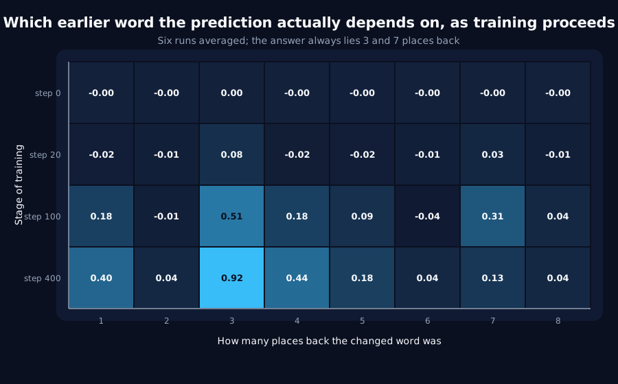
The measurement. Pick one scored position per held-out sequence, corrupt a single input token k places before it, and see how far accuracy at that position falls. Repeat for every offset from 1 to 8. Corruptions are drawn once per seed and reused at every training step, so every reading is paired with every other.

Kill test, fixed in advance: effective context is flat across the transition.

The ground truth, and the version of it that was wrong

synthetic-delayed-copy-v1 at lag 4 makes the target at position t equal to the input at t - 3. The obvious ground truth is therefore "offset 3, and nothing else".

That is wrong, and the first run of this pilot showed it. The sequence is periodic with period 4, so the inputs at t - 3, t - 7 and t - 11 are the same token. Every offset congruent to 3 modulo the lag is a valid source. Scoring only offset 3 as correct would have counted a solved model's dependence on offset 7 as a distraction. The check used here is whether dependence sits on {3, 7} and nowhere else.

Result: the dependence profile, step by step

Mean fall in accuracy when one token at each offset is corrupted, across 6 seeds. The accuracy midpoint is at step 86.7 [82.4, 91.0].

step	off 1	off 2	off 3	off 4	off 5	off 6	off 7	off 8
0 (untrained)	`-0.000`	`-0.004`	`+0.001`	`-0.000`	`-0.001`	`-0.000`	`-0.000`	`-0.000`
20	`-0.016`	`-0.008`	`+0.082`	`-0.023`	`-0.016`	`-0.009`	`+0.035`	`-0.008`
40	`-0.040`	`-0.030`	`+0.145`	`-0.043`	`-0.039`	`-0.037`	`+0.136`	`-0.039`
100	`+0.183`	`-0.008`	`+0.513`	`+0.182`	`+0.088`	`-0.039`	`+0.313`	`+0.040`
200	`+0.424`	`+0.090`	`+0.856`	`+0.421`	`+0.223`	`+0.087`	`+0.215`	`+0.073`
400	`+0.402`	`+0.043`	`+0.915`	`+0.437`	`+0.175`	`+0.042`	`+0.126`	`+0.044`

Bold columns are the two valid sources.

The model is looking in the right place 83 steps before its accuracy moves

endpoint	value
accuracy midpoint	`86.7` `[82.4, 91.0]`
first step where the largest drop is on a valid offset, and stays there	`3.3` `[0.6, 6.0]`
lead of that ranking	`+83.3` `[+80.6, +86.0]`
first step where total dependence clears `0.05`	`10.0` `[5.3, 14.7]`
lead of that threshold	`+76.7` `[+68.8, +84.6]`

The untrained model is the control, and it is flat. At step 0 every drop is within 0.004 of zero and the largest one lands on a valid offset in 2/6 runs, which is chance for 2 valid offsets out of 8. So the ranking is not a property of the architecture or the task; it appears within the first few updates.

And the threshold is not making the effect. The floor is itself an endpoint, so it was swept:

dependence floor	lead
`0.02`	`+80.0` steps
`0.05`	`+76.7`
`0.10`	`+65.0`
`0.20`	`+56.7`

A tenfold change in the floor moves the lead by a third and never near zero. The threshold-free ranking endpoint, which offset has the largest drop, needs no floor at all and gives the longest lead of the lot.

For scale, against every other leading indicator in this programme:

instrument	lead	cost
F2's decode probe	`+23.5` steps	`55.4%` of the training budget (J7)
K1's `global_norm`	`+30.8`	`0.15%`
M6's held-out bits	`+19.0`	already computed
this: which offset matters most	`+83.3`	8 extra forward passes per reading

It is the longest lead recorded here by a factor of nearly three. It is not free: it needs one forward pass per offset, but it needs no probe to be trained, no gradient buffer, and no eigendecomposition, and its cost scales with how many offsets you care to test rather than with the model.

The usual caution applies and is not negotiable. K1 showed the manoeuvre a lead gets spent on works just as well timed at random, and K2 showed the one real saving needs no detector. A longer lead does not change either. This is a measurement of when the model starts looking in the right place, not a demonstration that knowing it is worth anything.

The kill test does not fire, and the direction is a surprise

Effective context, the dependence-weighted mean offset, moves from 3.86 [3.45, 4.27] at its first determinate reading to 3.35 [3.21, 3.50] at the end, a change of -0.51 [-0.88, -0.13] that excludes zero. It narrows onto the correct offset rather than widening. The expected shape was a model that starts guessing from the nearest token and learns to look further back; what happens is that it looks in the right place almost immediately and then sharpens.

Half of a solved model's dependence is on tokens that cannot help it

At the end of training, the share of measurable dependence sitting on valid offsets is 0.479 [0.450, 0.508]. Offsets 1 and 4 carry +0.402 and +0.437, comparable to the correct offset's +0.915, and neither contains any information about the answer.

The likely reason is structural: the sequence is periodic, so corrupting any position breaks the pattern the recurrent state is tracking. A pure lookup would be unaffected. This is the same fact M1 reports from the other side, a zero-parameter cache model scores 1.0000 on this task and the GRU does not catch it in 2,000 steps. The network is not implementing the lookup; it is tracking the whole periodic structure, and paying for it in sensitivity to tokens that do not matter.

Verdict

The kill test does not fire. Effective context changes materially across training, narrowing by -0.51 [-0.88, -0.13].
The model's largest dependence sits on a valid copy source from the first few updates, 83.3 steps [80.6, 86.0] before its accuracy midpoint, with an untrained control that is flat and a threshold sweep that does not move the conclusion.
A solved model spends about half its measurable dependence on tokens that carry no information about the prediction being scored.
The anchor reproduced: the accuracy midpoint sits at 86.7, inside the published band.

Limits

Six seeds, one task, one width, one lag, one learning rate. The periodicity that creates the second valid offset is a property of this task's construction, and the dependence-on-useless- tokens result may be too.
Single-token corruption measures marginal dependence, not joint. A model that reads two positions redundantly will show a small drop at each, and this cannot distinguish that from genuinely weak dependence on both.
The corruption is a random replacement token, not a deletion or a mask. A different corruption would give a different scale, though the ranking endpoint is insensitive to scale by construction.
"Lead" here means lead over the accuracy midpoint on the same held-out batch, so it shares M6's limit: this is not an independent instrument in the way a probe on the hidden state is.
The eight offsets are a design choice. Offset 11 is also valid and was not probed, because probing it would have required restricting the scored positions further.

Terms on this page

Every piece of vocabulary this record uses, in plain language. Generated from the text above, so it cannot drift out of step with it.

accuracy: The fraction of answers a model gets right on questions it was not trained on.
architecture: The blueprint of a model: what components it has and how they connect. Two models can be the same size and completely different architectures.
gradient: The direction and amount by which each of a model's internal numbers should change to do slightly better. Training is repeatedly following it.
GRU: Gated Recurrent Unit. A compact design for processing sequences one item at a time, with internal switches controlling what it keeps in memory.
held-out: Data the model was never trained on, kept back specifically to test it. Scoring a model on data it has already seen measures memorisation, not learning.
hidden state: The model's working memory: the internal numbers it carries from one step of a sequence to the next.
kill test: A condition written down before running the experiment that says what result would make us abandon the idea. Fixing it in advance is what stops a disappointing result being reinterpreted as an encouraging one.
learning rate: How big a step training takes each time it updates the model. Too small and nothing happens; too big and it never settles.
probe: A small separate model trained to read information out of a bigger model's internals, used as a measuring instrument rather than as a product.
recurrent: A design that reads a sequence one item at a time, carrying memory forward. The main alternative is attention, which looks at everything at once.
seed: The number that fixes all the randomness in a training run. Same seed, same run. Running several seeds is how you tell a real effect from a lucky one.
width: How many internal numbers a model uses at each layer. The usual way we vary model size in these experiments.