How do you know a fine-tuned AI model is actually better?

You measure it. Hold out a portion of the client's real examples so the model never sees them during training, score the plain base model on those held-out questions first, fine-tune, then score again on the identical questions with identical scoring. The difference is the lift. Because the only thing that changed is the fine-tune, the improvement is attributable to it.

Does fine-tuning actually improve accuracy, or is the base model already good enough?

It depends on the task and, critically, on how much data you have. On a public benchmark of 510 lawyer-annotated commercial contracts, a base Qwen3-4B extracted short contract fields at 62.2% accuracy. Fine-tuned on 396 examples it reached 83.5-85.4%, a lift of 21.3 to 23.2 points across three runs. The same model trained on only 48 examples produced a lift inside the noise floor, so the amount of data was the deciding factor rather than the model's ceiling.

How much of our own data do we need to fine-tune a model?

Fewer examples than most people expect, but more than a handful. In our contract-extraction measurements, 48 training examples produced no measurable improvement while roughly 400 produced a 22-point gain. The honest answer for any specific case is that it depends on how varied and how consistent the examples are, which is what a paid readiness assessment measures on the client's own corpus.

Why can't you just use a public AI benchmark score?

Public benchmarks measure general ability on standardised tests, not your work. A model that scores well in the abstract can still be mediocre at reading your contracts or following your policies. Public benchmarks are also increasingly targeted during training, so a high score can reflect test preparation as much as capability. The only benchmark that answers your question is built from your own tasks.

Research record 44 of 47

The Detector Was Never the Problem

By Joshua Bolick, Awareness Software Group ~16 min read August 2026

Ongoing research. This is an experimental result from active work, not a settled conclusion. The numbers are what we measured and the method is described so you can judge it, but the programme is still running and later experiments may revise what it means. More about this programme.

In plain English

What we asked. In an earlier experiment we tried to use our best early-warning signal to make training cheaper, and it failed for an embarrassing reason: computing the signal cost more than half of the entire training budget, which was about thirteen times what it saved. We wrote at the time that a cheaper detector with the same warning would change the arithmetic. This experiment goes and gets one.

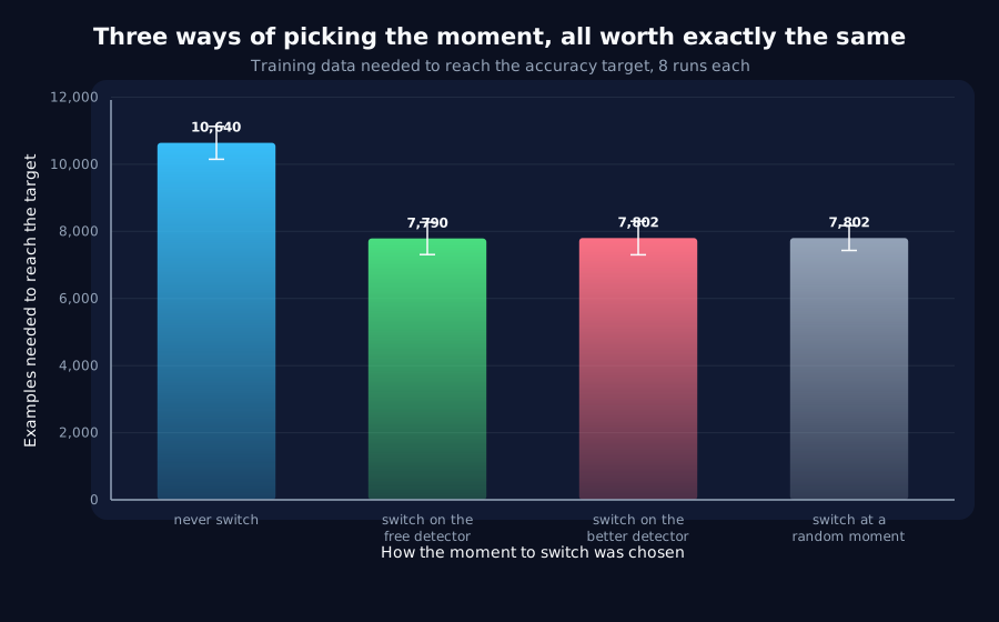
What we found. We found two, both far cheaper. One costs about nine percent of a training step and the other is effectively free, about a sixth of one percent, against the old signal's fifty five percent. And the outcome is identical. Switching to a cheaper training setting part way through saves about twenty seven percent of the data either way, but making the switch when our signal fires is no better than making it at a random moment. So the cost of the detector was never what made this fail. The moment it identifies simply is not worth knowing.

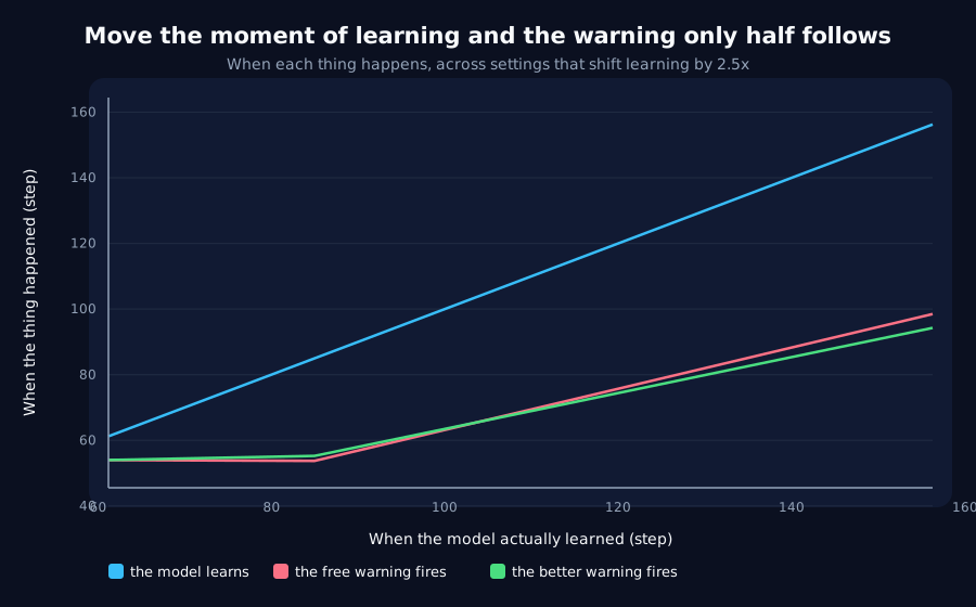
Why it matters. The more useful half is why. A warning that always fires at the same point will look useful if you only ever test it in one setting, because its apparent head start is just the gap between that fixed point and the average moment of learning. The way to tell is to move the event, so we changed the training speed until models learned anywhere from step sixty to step one hundred and fifty six, and asked whether the warnings moved with them. They covered about half the distance. That means the head start is not something you can plan around: it is about sixty steps when learning is slow and about seven when it is fast. Two of our own controls also failed during this experiment, both in the direction that would have made the result look better, and both were caught by a small practice run before the real one. One of them was a safety limit we had added to stop the detector looking good too easily, which turned out to be manufacturing the very head start it was meant to protect.

The rest of this page is the technical record: the design, every number, and the limits. It is written for a reviewer, and you do not need it to have understood the result above.

New here? How to read a research record

Start at the verdict. Every record states, before the experiment was run, what result would have made us abandon the idea. That is the "kill test". Then it says whether the test fired. Nothing gets reinterpreted after the fact.
Numbers in square brackets are uncertainty. 23.4 [18.1, 28.7] means our best estimate is 23.4 and the true value is probably somewhere in that range. If a range includes zero, we cannot claim an effect.
Negative results are kept. Roughly half of what is published here says an idea did not work, including several of our own. Those pages are not failures, they are the output. Work that only publishes what worked is not measuring anything.
Read the Limits section. Every record ends with what it does not show. It is the most honest part of any experiment and usually the shortest.
Pro tip: the figures near the top are designed to carry the result on their own. If you read nothing else, read the caption under each one, which says what it shows and what to take from it.

EXPLORATORY. Not a preregistered study. Local CPU, 44 training runs, no GPU, no cost.

Program v2 Bucket K, item K1. Decisive computation: analysis/spend_the_cheap_lead.py. Output: analysis/spend_the_cheap_lead.json. Reproduce with python analysis/spend_the_cheap_lead.py, or re-derive every endpoint, including the tracking grades, from the saved series with --reuse.

The question

J7 tried to spend F2's decode probe and lost by an order of magnitude. Cutting the batch at the crossing saved a real 22% of data-to-target, a random-timed cut saved the same, and detecting the moment cost 55.4% of the training budget against a 2,460-sample saving. J7's own record named the escape hatch: "a cheaper detector with the same lead would change the arithmetic."

**Three ways of picking the moment, all worth exactly the same.** Earlier we found that switching a model to a cheaper training setting partway through saves real data, but that picking the moment with our best early-warning signal was no better than picking at random, and the signal cost more to compute than it saved. So we tried two much cheaper signals, one of which is effectively free. Lower bars are better. The grey bar is the honest comparison: the same switch made at a moment chosen at random. The switch is worth having, about 27% less data than never switching. But the three switched bars are the same height, including the random one. The cheap signals really are cheap, one of them costs about a sixth of one percent of a training step against the old signal's fifty-five percent, and it changes nothing at all. The cost of the detector was never what made this fail: the moment it identifies simply is not worth knowing.

**Move the moment of learning and the warning only half follows.** A warning that always fires at the same moment will look useful if you only ever test it in one setting: its apparent head start is just the gap between that fixed moment and the average moment of learning. The way to tell is to move the event. Here we changed the training speed so the model learns anywhere from step 61 to step 156, and asked whether the warnings moved with it. The blue line is the event itself, so it is the shape a perfect warning would trace. Both warnings move in the right direction and cover only about half the distance. That means the head start is not a fixed quantity you can plan around: it is about 60 steps when learning is slow and about 7 when it is fast. A warning quoted without the setting it was measured in is not telling you what it appears to. This is the third time in this project that a promising early signal has failed the same check, which is why moving the event is now something we do before believing any of them.

K1 walks through that hatch. It swaps the expensive probe for gradient statistics that cost almost nothing and, in one case, lead further.

Kill test, fixed in advance: at a compute-matched budget the gradient-timed switch does not beat the random-timed switch.

The premise was wrong, and that was free to find out

Bucket K proposed G1's off_top:variance as the cheap detector, on the grounds that it is "a variance accumulator over gradients the optimiser has already computed."

It is not. off_top is the part of the gradient lying outside the leading direction, so computing it requires that direction, which means an eigendecomposition of the gradient buffer's Gram matrix on every step. The genuinely free statistic is A11's global_norm:variance, one reduction over a vector that already exists.

So both were run, and both were timed rather than assumed:

Instrument	Cost per training step
`global_norm`	`0.15%`
`off_top`	`9.0%`
J7's decode probe	`55.4%`

The estimate that went into the backlog entry was ~45% for off_top. Measuring beat asserting in both directions, which is J7's own rule applied to J7's own successor.

Result: the kill test fires, and the cost was never the problem

Eight test seeds, matched budget of 57,600 samples, batch cut 4x at the alarm.

Arm	Final accuracy	Samples to target
control	`0.9906` `[0.9893, 0.9920]`	`10,640` `[10,150, 11,130]`
norm-timed	`0.9852` `[0.9806, 0.9898]`	`7,790` `[7,308, 8,272]`
offtop-timed	`0.9846` `[0.9800, 0.9891]`	`7,802` `[7,302, 8,302]`
random-timed	`0.9853` `[0.9820, 0.9885]`	`7,802` `[7,432, 8,172]`

The batch cut saves 26.8% of data-to-target and the timing contributes nothing. All three switched arms are indistinguishable; the random-timed arm lands on 7,802, the same as offtop-timed to the sample.

The instrument now pays for itself easily: global_norm spends 5 samples to save 2,850, and it does not matter, because the saving is not attributable to the timing. A random switch collects it for free.

J7's escape hatch is closed. Making the detector cheaper does not rescue the manoeuvre, because the detector's cost was never what killed it.

Why the timing is worth nothing: the alarm is half a clock

The kill test says the timing does not help. The tracking test says why, and it is the more useful half of this record.

An alarm that fires at a fixed step has a "lead" equal to the mean transition minus that step, which looks exactly like a detector until the transition is deliberately moved and the alarm is asked to follow. So the learning rate was swept to move the transition 2.5x:

Learning rate	Transition	`global_norm` alarm	`off_top` alarm	Lead
`0.002`	`156.2`	`98.5`	`94.2`	`~60`
`0.005`	`85.0`	`53.8`	`55.2`	`~31`
`0.012`	`61.2`	`54.0`	`54.0`	`~7`

Both alarms follow only about half the movement: slope +0.525 (r = +0.878) for global_norm and +0.469 (r = +0.865) for off_top. They are neither detectors nor clocks; they are partly anchored near initialisation.

The consequence is visible in the last column. At the fast setting the lead collapses to 7 steps. As a fraction of the transition time the lead runs 38% at the slow setting and 11% at the fast one, averaging 28%, so the warning is not a fixed budget of steps, and knowing how much warning you have requires already knowing roughly when the transition is. That is D4's finding in a third place, on a different family of statistics, and it is also J5's: a lead quoted without its setting is not a property of the indicator.

The two corrections this record is really about

The random control was broken, and it was broken in the direction that passes the test. The first version drew each seed's random switch step from that same seed's observed alarms, so alarm == random in 7 of 8 seeds. The kill test was comparing an arm against a copy of itself, which it passes by construction. It now draws leave-one-out from the pooled alarms of other seeds. Matched in distribution and independent of the run are both required, and only the first is obvious.

A constant added to protect the result was creating it. A WARMUP floor of 60 steps was added so that a detector could not fire trivially early. On this configuration the transition is at step 80-90, so 60 left almost no room, and every alarm at every usable threshold fired on the boundary itself, a clock whose apparent lead was an artifact of where the boundary had been put. The selection rule then made it worse by picking the threshold with the longest lead, which rewards firing as early as permitted. Removing the floor, the same alarms fire at 50-66 with real spread and a ~30-step lead. The selection rule now rejects any threshold whose firing step does not vary across the selection seeds.

Both were caught by a smoke test at reduced scale before the full run, which is the only reason they are corrections rather than a published result.

Verdict

The kill test fires. No gradient-timed switch beats a random-timed one at a matched budget.
The cheap indicator is genuinely cheap (0.15% of a step against the probe's 55.4%) and that changes nothing. J7's escape hatch is closed: the detector's cost was not the problem.
The manoeuvre is real and the timing is not. Cutting the batch is worth 26.8% of data-to-target and can be had for free at any moment.
The mechanism is partial tracking. Both statistics follow only about half the transition's movement, so their lead shrinks to 7 steps where the transition is fast. A "lead" measured at one setting is not a property of the indicator.
A standing check earns its place: before quoting any indicator's lead, move the event and see whether the indicator follows. Three items in this programme have now failed that check.

Limits

Eight test seeds, four selection seeds, one task, one width, one manoeuvre. The batch cut is J7's and was not varied; a different cheaper regime might interact with timing differently.
The tracking sweep is three learning rates on four seeds. The slope is estimated from twelve points across a 2.5x change in transition step, which is enough to separate 0.5 from 1.0 but not to pin the exponent.
The transition is quantised by 5-step logging. Within a single setting it takes only two distinct values here, which is why the tracking test varies the learning rate rather than relying on within-setting correlation. A within-setting correlation of +0.000 was computed on the first run and is not evidence of anything, for exactly this reason.
Instrument costs are wall-clock ratios measured in one process under a CPU duty-cycle throttle. The ratio is meaningful and portable; the absolute milliseconds are not.
The alarm rule is one family, a rolling variance against its own running median. A different rule on the same statistics might track better, and nothing here rules that out.

Terms on this page

Every piece of vocabulary this record uses, in plain language. Generated from the text above, so it cannot drift out of step with it.

accuracy: The fraction of answers a model gets right on questions it was not trained on.
compute-matched: Comparing two methods by giving them the same amount of computing power rather than the same number of steps. A method that takes twice as long per step should not get twice the compute for free.
gradient: The direction and amount by which each of a model's internal numbers should change to do slightly better. Training is repeatedly following it.
kill test: A condition written down before running the experiment that says what result would make us abandon the idea. Fixing it in advance is what stops a disappointing result being reinterpreted as an encouraging one.
learning rate: How big a step training takes each time it updates the model. Too small and nothing happens; too big and it never settles.
probe: A small separate model trained to read information out of a bigger model's internals, used as a measuring instrument rather than as a product.
seed: The number that fixes all the randomness in a training run. Same seed, same run. Running several seeds is how you tell a real effect from a lucky one.
slope: How steeply one quantity changes as another does. A slope of one between a warning and the event it predicts means the warning shifts exactly in step with the event.
variance: How spread out a set of numbers is. Rising variance in a signal means it is becoming more erratic.
width: How many internal numbers a model uses at each layer. The usual way we vary model size in these experiments.