How do you know a fine-tuned AI model is actually better?

You measure it. Hold out a portion of the client's real examples so the model never sees them during training, score the plain base model on those held-out questions first, fine-tune, then score again on the identical questions with identical scoring. The difference is the lift. Because the only thing that changed is the fine-tune, the improvement is attributable to it.

Does fine-tuning actually improve accuracy, or is the base model already good enough?

It depends on the task and, critically, on how much data you have. On a public benchmark of 510 lawyer-annotated commercial contracts, a base Qwen3-4B extracted short contract fields at 62.2% accuracy. Fine-tuned on 396 examples it reached 83.5-85.4%, a lift of 21.3 to 23.2 points across three runs. The same model trained on only 48 examples produced a lift inside the noise floor, so the amount of data was the deciding factor rather than the model's ceiling.

How much of our own data do we need to fine-tune a model?

Fewer examples than most people expect, but more than a handful. In our contract-extraction measurements, 48 training examples produced no measurable improvement while roughly 400 produced a 22-point gain. The honest answer for any specific case is that it depends on how varied and how consistent the examples are, which is what a paid readiness assessment measures on the client's own corpus.

Why can't you just use a public AI benchmark score?

Public benchmarks measure general ability on standardised tests, not your work. A model that scores well in the abstract can still be mediocre at reading your contracts or following your policies. Public benchmarks are also increasingly targeted during training, so a high score can reflect test preparation as much as capability. The only benchmark that answers your question is built from your own tasks.

Research record 33 of 39

We Let It Learn How to Combine Them

By Joshua Bolick, Awareness Software Group ~11 min read August 2026

Ongoing research. This is an experimental result from active work, not a settled conclusion. The numbers are what we measured and the method is described so you can judge it, but the programme is still running and later experiments may revise what it means. More about this programme.

In plain English

What we asked. We have two independent early warnings that a model is about to improve. An earlier experiment found that requiring both to agree buys nothing at all. The fair objection is that we combined them in the crudest possible way, by simply demanding both cross a line. So here we gave a small model both signals and let it learn how much to trust each.

What we found. It appeared to work: the learned version beats our earlier hand-set rule. But we also ran it with only the better of the two signals, and that version captures almost all of the improvement. What the second signal adds is one run out of twelve at three settings, and at a fourth it makes things worse. The model itself learned to weigh the first signal between seven and thirty-nine times more heavily than the second.

Why it matters. The genuinely useful discovery was accidental. Since a model given only one signal beat our earlier rule using that same signal, our earlier result was being held back not by the signal but by how crudely we had set its cut-off. The numbers we published for it were a floor rather than a ceiling. We should also say plainly that four earlier versions of this experiment produced confident-looking negative results that were simply broken, each for a different and unobvious reason. We only caught them because we had built a check that had to succeed if the setup was sound. How you set an alarm is not a detail.

The rest of this page is the technical record: the design, every number, and the limits. It is written for a reviewer, and you do not need it to have understood the result above.

New here? How to read a research record

Start at the verdict. Every record states, before the experiment was run, what result would have made us abandon the idea. That is the "kill test". Then it says whether the test fired. Nothing gets reinterpreted after the fact.
Numbers in square brackets are uncertainty. 23.4 [18.1, 28.7] means our best estimate is 23.4 and the true value is probably somewhere in that range. If a range includes zero, we cannot claim an effect.
Negative results are kept. Roughly half of what is published here says an idea did not work, including several of our own. Those pages are not failures, they are the output. Work that only publishes what worked is not measuring anything.
Read the Limits section. Every record ends with what it does not show. It is the most honest part of any experiment and usually the shortest.
Pro tip: the figures near the top are designed to carry the result on their own. If you read nothing else, read the caption under each one, which says what it shows and what to take from it.

EXPLORATORY. Not a preregistered study. Local CPU, no training at all, no GPU, no cost.

Program v2 Bucket I, item I4. Decisive computation: analysis/fitted_combiner.py. Output: analysis/fitted_combiner.json. Reproduce in seconds with python analysis/fitted_combiner.py, reading the series G6 committed.

The question

G6 closed the two simplest ways to combine this programme's two leading indicators: both must fire, either may fire, and named the version it did not test in its own Limits: a fitted combiner. That is the version an engineer would build, and the version that is easy to overfit on twelve runs.

**Learning how to weigh two signals does not rescue the second one.** An earlier experiment found that demanding two warning signals agree buys nothing. The obvious objection is that it used the crudest possible way of combining them, so here a small model is given both signals and left to learn how much to weigh each. The bottom line is that earlier hand-set rule; the middle line is the same learned model given only the better signal, which is the comparison that isolates what the second one contributes. The learned model does beat the old hand-set rule, but the middle line shows almost all of that comes from choosing a better cut-off rather than from having a second signal. Between the top two lines the gap is one run in twelve at three widths, and it goes the wrong way at the widest. The useful discovery is the bottom line: our earlier result was held back by a coarse choice of cut-off, so the numbers we published for it were a floor, not a ceiling.

Kill test: the fitted combiner does not beat the decode probe alone at matched false-alarm rate on held-out runs.

This runs entirely on G6's saved per-step series, which is the payoff of that pilot's --reuse design.

Result: the letter and the intent diverge again

A logistic model on the two standardised indicator values, fitted on 6 selection runs and scored once on 12 disjoint confirmation runs, at each horizon:

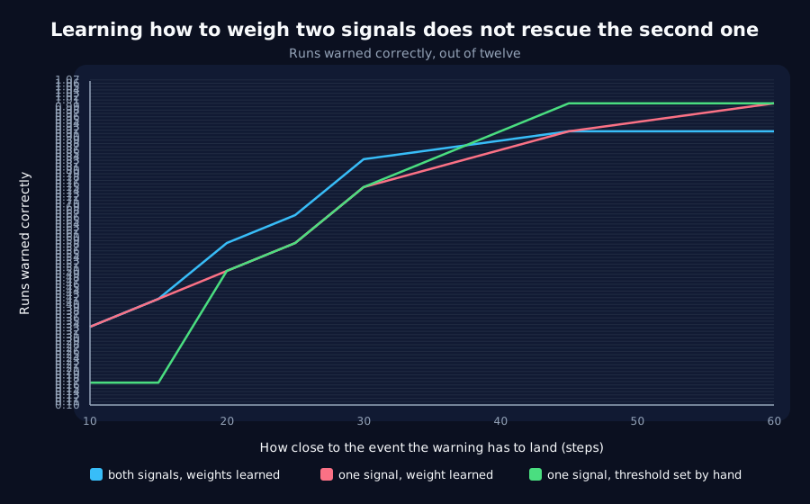
Horizon	Fitted pair	Fitted probe alone	G6's hand-set probe	Pair at matched false-alarm rate
10	`0.33`	`0.33`	`0.17`	`0.08`
15	`0.42`	`0.42`	`0.17`	`0.08`
20	`0.58`	`0.50`	`0.50`	`0.58`
25	`0.67`	`0.58`	`0.58`	`0.67`
30	`0.83`	`0.75`	`0.75`	`0.83`
45	`0.92`	`0.92`	`1.00`	`0.92`
60	`0.92`	`1.00`	`1.00`	`1.00`

By its letter the kill test fails. At horizons 20, 25 and 30 a fitted combiner beats G6's hand-thresholded probe at a matched false-alarm rate.

By its intent it fires. A fitted model differs from G6's rule in two ways at once: it has a second signal, and it has a different threshold family. The probe-only arm holds the second constant, and it is the comparison that isolates the second signal:

Horizon	Pair	Probe alone	Difference
10, 15, 45	,	,	`+0.00` (0 runs)
20, 25, 30	,	,	`+0.08` (+1 run of 12)
60	`0.92`	`1.00`	`-0.08` (-1 run of 12)

The second signal is worth at most one run in twelve, at three of seven horizons, and costs one run at a fourth. The fitted weight on the probe is 7x to 39x the weight on the gradient statistic across horizons. Nearly all of the gain over G6 is the threshold family, not the second signal.

The overfitting check, selection minus confirmation hit rate, is +0.024 [-0.100, +0.147] across horizons, so the fitted model is not obviously memorising its six runs. That check is what makes the one-run margins readable at all, and it does not make them large.

Four broken instruments, and the check that caught them

This record is mostly about how hard the alarm rule was to get right. Four versions produced a confident-looking zero before one worked. Each is recorded in the script at the site of the thing that caused it.

An absolute probability grid (0.05, 0.10, ... 0.95). A model fitted on labels positive for 30 of 846 rows assigns probabilities in a narrow low band, 0.002 to 0.27 here, so no threshold in that grid sits between "fires at the first eligible step in every run" and "never fires at all". Every arm scored 0.00.
G6's multiplicative grid, applied to the probability. A multiplier is only meaningful on the scale it was designed for. The sigmoid compresses the top of the range, so max x 1.5 still fires immediately and max x 20 is unreachable. Same gap, same zero.
Fitting on every row rather than only pre-event rows. The probe is high just before the transition and high forever after it, and only the former is labelled positive, so the fit returned a negative probe weight: true of that training set and useless as a forward alarm. A first-alarm rule is decided entirely before the event, so post-event rows are not part of the decision problem.
An 11-point threshold grid. Standardising a feature is an affine map, so for every threshold on the raw probe an equivalent one exists exactly. A coarse grid can still miss it, and did: the probe-only arm topped out at 0.33 against the hand-set rule's 1.00.

The check that caught all four: a probe-only arm fitted the same way is a monotone function of the probe, so its frontier must reach the hand-thresholded probe's performance. It does, at every horizon, once the parameterisation is right.

That check runs on the selection runs, not the confirmation runs. This analysis was iterated four times; checking a diagnostic against the held-out set and stopping when it looks right is precisely the leak the split exists to prevent.

Verdict

Combining these two indicators is closed, now in its strongest form as well as its simplest.
The apparent win over G6 is the threshold family. median + k x IQR on a fine grid finds better operating points than calibration max x multiplier on a coarse one, and that has nothing to do with having two signals. This is worth more than the null: G6's own numbers were limited by its threshold grid, and its 20/25/30-step reliability is a floor rather than a ceiling.
An alarm rule is not a detail. Four of five parameterisations here produced a decisive-looking negative from an instrument that was not measuring the signal.

Limits

6 selection and 12 confirmation runs, one task, one width, one architecture, G6's population exactly, with its limits inherited.
A logistic model on two levels is the simplest fitted combiner. Rates of change, longer feature histories, or a nonlinear model are untested, and the non-monotonicity that broke attempt 3 is a hint that a rate feature might behave differently.
The one-run margins are one run. With twelve confirmation runs the resolution of any hit rate is 0.083, so "+1 run at three horizons" is at the edge of what this population can resolve, and is reported as such rather than as an effect.
The overfitting check compares selection with confirmation on the same seeds throughout; it is a sanity check, not a generalisation estimate.

Terms on this page

Every piece of vocabulary this record uses, in plain language. Generated from the text above, so it cannot drift out of step with it.

architecture: The blueprint of a model: what components it has and how they connect. Two models can be the same size and completely different architectures.
false-alarm rate: How often a warning system goes off when nothing is actually happening. Any detector can be made to fire early by making it twitchier, so a lead time only means something alongside this number.
gradient: The direction and amount by which each of a model's internal numbers should change to do slightly better. Training is repeatedly following it.
held-out: Data the model was never trained on, kept back specifically to test it. Scoring a model on data it has already seen measures memorisation, not learning.
held-out set: Data or runs kept aside and not used while choosing what to report, so a finding can be tested on something it was not tuned against.
kill test: A condition written down before running the experiment that says what result would make us abandon the idea. Fixing it in advance is what stops a disappointing result being reinterpreted as an encouraging one.
overfitting: When a model learns the training data specifically rather than the pattern behind it, and so does well in training and badly on anything new.
probe: A small separate model trained to read information out of a bigger model's internals, used as a measuring instrument rather than as a product.
reliability: How often something works on an individual case, as opposed to how well it does on average. The two can differ a lot, and only one of them tells you what to expect next time.
seed: The number that fixes all the randomness in a training run. Same seed, same run. Running several seeds is how you tell a real effect from a lucky one.
width: How many internal numbers a model uses at each layer. The usual way we vary model size in these experiments.

About this record. This page is the write-up of an experiment we ran ourselves. Every number on it comes from a run we recorded, and the script that produced each one is named in the text above. We publish these results and the data behind them here, including the ones that went against what we expected.

Why we do this. The same care shown above is what we apply to client work. We build custom AI models that you own and run yourself, using our own platform, and the reason we publish research like this is that a model is only worth what its evaluation is worth. If a supplier cannot show you the experiments that went against them, you cannot check the ones that went their way.

All research from this programme →