How do you know a fine-tuned AI model is actually better?

You measure it. Hold out a portion of the client's real examples so the model never sees them during training, score the plain base model on those held-out questions first, fine-tune, then score again on the identical questions with identical scoring. The difference is the lift. Because the only thing that changed is the fine-tune, the improvement is attributable to it.

Does fine-tuning actually improve accuracy, or is the base model already good enough?

It depends on the task and, critically, on how much data you have. On a public benchmark of 510 lawyer-annotated commercial contracts, a base Qwen3-4B extracted short contract fields at 62.2% accuracy. Fine-tuned on 396 examples it reached 83.5-85.4%, a lift of 21.3 to 23.2 points across three runs. The same model trained on only 48 examples produced a lift inside the noise floor, so the amount of data was the deciding factor rather than the model's ceiling.

How much of our own data do we need to fine-tune a model?

Fewer examples than most people expect, but more than a handful. In our contract-extraction measurements, 48 training examples produced no measurable improvement while roughly 400 produced a 22-point gain. The honest answer for any specific case is that it depends on how varied and how consistent the examples are, which is what a paid readiness assessment measures on the client's own corpus.

Why can't you just use a public AI benchmark score?

Public benchmarks measure general ability on standardised tests, not your work. A model that scores well in the abstract can still be mediocre at reading your contracts or following your policies. Public benchmarks are also increasingly targeted during training, so a high score can reflect test preparation as much as capability. The only benchmark that answers your question is built from your own tasks.

Research record 15 of 35

Predicting When a Model Will Learn

By Joshua Bolick, Awareness Software Group ~16 min read August 2026

Ongoing research. This is an experimental result from active work, not a settled conclusion. The numbers are what we measured and the method is described so you can judge it, but the programme is still running and later experiments may revise what it means. More about this programme.

In plain English

What we asked. Models we study spend a long time getting nowhere and then suddenly get the task right. We wanted two things: a map of when that moment arrives across the settings people actually choose when training, and a warning signal that could tell us it was coming.

What we found. Both. The map is smooth and predictable, and one of the three settings we varied turns out not to matter at all. For the warning, we found one that works: how much the training signal wobbles from step to step starts rising before the model learns, in every single run we could test it on, and it shifts when we deliberately move the moment of learning. It is also free, because it reads a number training already produces.

Why it matters. There is a well-known theory that predicts exactly this, and our result only half matches it. The theory says two things should happen before the jump and we could only confirm one, with the other two measurements inconclusive for reasons to do with our instrument rather than the model. So we have something useful and we are not claiming to know why it works. The honest summary is that we found a detector, not an explanation.

The rest of this page is the technical record: the design, every number, and the limits. It is written for a reviewer, and you do not need it to have understood the result above.

New here? How to read a research record

Start at the verdict. Every record states, before the experiment was run, what result would have made us abandon the idea. That is the "kill test". Then it says whether the test fired. Nothing gets reinterpreted after the fact.
Numbers in square brackets are uncertainty. 23.4 [18.1, 28.7] means our best estimate is 23.4 and the true value is probably somewhere in that range. If a range includes zero, we cannot claim an effect.
Negative results are kept. Roughly half of what is published here says an idea did not work, including several of our own. Those pages are not failures, they are the output. Work that only publishes what worked is not measuring anything.
Read the Limits section. Every record ends with what it does not show. It is the most honest part of any experiment and usually the shortest.
Pro tip: the figures near the top are designed to carry the result on their own. If you read nothing else, read the caption under each one, which says what it shows and what to take from it.

EXPLORATORY. Not a preregistered study. Local CPU, 82 training runs, no GPU, no cost.

Program v2 tier 3, item F1. Decisive computation: analysis/critical_slowing.py. Output: analysis/critical_slowing.json. Reproduce with python analysis/critical_slowing.py in about fifty minutes on a throttled laptop CPU. The numbers below reproduced exactly on a second execution.

The question

Dynamical-systems theory makes a specific, falsifiable prediction about a system approaching a tipping point: critical slowing down. As a stability boundary nears, the system recovers more slowly from perturbation, so its fluctuations grow and become more autocorrelated before the jump. Rising variance plus rising lag-1 autocorrelation is the standard early-warning battery, used on climate records, ecosystems and physiological time series.

**An early warning that moves when the event moves.** Each dot is one training run. Along the bottom is the moment the model suddenly learned the task, which we moved deliberately across a wide range by changing ordinary training settings. Up the side is when an alarm went off, watching only how much the training signal was wobbling. The dashed line marks an alarm arriving exactly at the moment of learning, so dots below it are genuine advance warning. The alarm was tuned in advance to go off no more than one time in five on scrambled data containing no real warning. The dots sit just below the line and follow it closely across the whole range. That is the test an earlier candidate failed: a signal that always fires at the same early moment will appear to lead by a lot and is useless, because its apparent warning is just the gap to a fixed point. This one moves with the event, firing about 25 steps ahead in every one of the 49 runs it was measured on. It also costs nothing to compute, because it reads a quantity training already produces.

**When the model learns, across the settings you actually choose.** Every cell is a pair of training runs at one combination of settings, and the number is the step at which the model suddenly learned the task. Darker means later. The two settings shown are the two that a practitioner picks by hand for every training job: how big a step to take, and how many examples to look at before taking it. Blank cells are combinations where the model never learned within the budget. The moment of learning is not a fixed property of the problem. It moves by hundreds of steps across ordinary settings, and it moves smoothly and predictably: slower learning rates and larger batches push it later, with no sharp boundary anywhere in the grid. That predictability is what makes the map useful, and it is also what makes the early-warning question worth asking, because the answer cannot simply be read off the settings when the settings are not known in advance.

It was the last leading-indicator candidate in the program, the only theory-backed one, and it uses a different class of signal from everything that failed: temporal fluctuation statistics rather than D4's weight spectra or v1's representation geometry.

Kill test, from docs/research-program-v2.md: no early-warning statistic beats a random-time-matched detector on lead time at fixed false-alarm rate across ten seeds.

Part A: the phase diagram

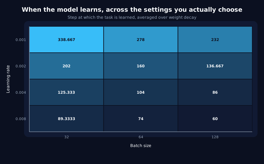
Learning rate x batch size x weight decay, two seeds each, with transition step, sharpness and expansion magnitude as order parameters. All 36 cells solved 2/2, and the transition spans 280 steps (60 to 340).

Axis	Range	Effect on transition step
Learning rate	`0.001` → `0.008` (8x)	`338` → `88` at batch 32. Dominant.
Batch size	`32` → `128` (4x)	`338` → `232` at lr `0.001`. Substantial.
Weight decay	`0.0` → `0.1` (100x)	mean `157.0` → `157.3`. Nothing.

Weight decay is not a lever on transition timing. Across a hundredfold range the mean transition moves by three tenths of a step, which is below the four-step resolution of the evaluation grid. That is a clean negative worth having: it removes an axis from every future sweep.

The map is smooth. There is no boundary anywhere in the grid, no cell where the transition fails to appear, and no discontinuity, timing moves gradually and monotonically with both live axes.

The expansion magnitude is invariant. Across all 36 cells it sits between 0.1999 and 0.2156, a spread of under 8% while transition timing moves by a factor of 5.7. The confirmed phenomenon's size does not depend on any of the three settings a practitioner tunes. (This endpoint is a max-minus-baseline quantity, which the program's standing rule says is positive under noise by construction; it is reported for mapping only and no claim here rests on it.)

Part B: the early-warning battery

Four statistics on the per-step training loss and gradient norm: rolling variance and lag-1 autocorrelation of within-window detrended residuals. Detrending first matters more than the choice of statistic: training loss falls steeply, so raw within-window variance measures the slope rather than the fluctuations, and critical slowing is a claim about the fluctuations.

49 of 82 runs eligible, 33 excluded. A detector needs history to calibrate on, so runs whose transition lands inside the calibration window plus one rolling window cannot be tested. Every exclusion is a fast cell. This is a limitation of the method, not of this pilot: the sooner a transition arrives, the less room any such detector has.

Statistic	Detect	Surrogate	Lead	Slope	`r`	Verdict
`gradient:variance`	100%	18%	`+25.5` `[21.5, 29.5]`	`0.89`	`+0.98`	passes all three
`loss:autocorrelation`	24%	18%	`-103.3` `[-201.6, -5.1]`	`2.11`	`+0.80`	fails
`gradient:autocorrelation`	22%	39%	`-48.9` `[-124.0, +26.2]`	`0.94`	`+0.50`	untested
`loss:variance`	0%	18%	,	,	,	fails

The result: gradient variance is a leading indicator

It clears all three controls:

Fixed false-alarm rate. Detects in 100% of runs at a threshold where a surrogate, the same run's fluctuations shuffled in time, destroying autocorrelation and the ordering of fluctuation size while preserving the trend, the marginal distribution and the scale, alarms on 18%.
Beats the random-time-matched detector by a wide margin (+25.5 against -191.0).
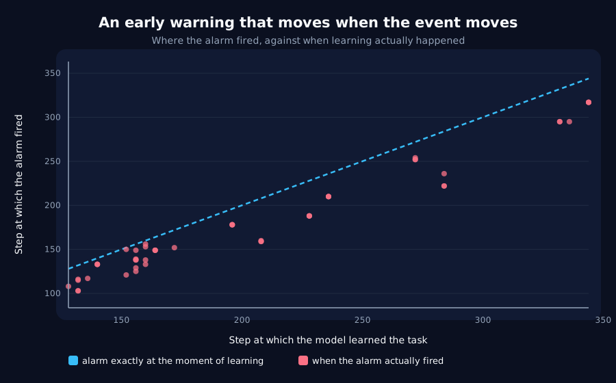
It follows the transition. Slope 0.89 at correlation +0.98, with the alarm spanning 214 steps against the transition's 216. This is the control D4 failed, and the reason that record exists.

It leads in 49 of 49 runs, and it is cheap: the gradient norm is already computed by clip_grad_norm_, so this needs no held-out labels, no probe fit, and no extra forward pass. That is the property F2's decode probe lacks.

The lead is proportional, not a fixed horizon

With slope b, lead = (1-b) x transition - c, so at b = 0.89 the lead is about 11% of the transition time rather than a constant.

Transition	Mean lead
Earlier than step 200 (n=28)	`+17.2`
Step 200 or later (n=21)	`+36.7`
Range across all 49	`+2` to `+62`

The minimum lead is 2 steps. The mean is comfortably positive and every run leads, but this is not a guaranteed warning horizon, and a use that needs a fixed number of steps of notice will not get one. Reporting +25.5 alone would overstate it.

This is a much milder proportionality than D4's, where b ≈ 0.3 made the "lead" roughly 70% of the transition time and therefore useless. At b = 0.89 most of the alarm's position is genuinely tracking the event. But it is proportional, and the record says so.

The theory is only half confirmed

Critical slowing down predicts both rising variance and rising autocorrelation. Only the first is present, and only on one of the two series:

gradient:autocorrelation is untested, not failed. Its threshold sweep never reached the false-alarm budget, at the strictest threshold it still alarmed on 39% of surrogates, so its detection rate is not comparable with the others. The cause is the instrument: a multiplicative threshold is the wrong parameterisation for a statistic bounded in [-1, 1] and sitting near zero. Recording it as a negative would repeat the error the vanilla RNN was recorded untested to avoid.
loss:variance alarms in 0% of real runs at a threshold where surrogates alarm 18%, so shuffled loss residuals are more alarm-prone than real ones. Loss variance does not rise before the transition.
loss:autocorrelation detects barely above its own false-alarm rate (24% against 18%).

So: a usable early warning exists, and the mechanism attributed to it does not follow. The honest reading is that gradient-norm fluctuations grow as the model begins to move, which is consistent with critical slowing down but equally consistent with the much duller explanation that the model is already changing before accuracy: a coarse, thresholded readout, registers it. That duller explanation is what F2 established directly, and F1 does not distinguish the two.

Do not describe this as confirming critical slowing down. It confirms a detector.

Verdict: the kill test does not fire

CORRECTION, 2026-08-23. The 49 of 49 reliability figure below is a property of this study's run population, not of its detector. F1 excluded 33 of 82 runs whose transitions landed too early to calibrate against, and every exclusion was a fast cell, so what remained was the slower half, where the alarm has the most room to fire early. A11 ran the same statistic on a differently filtered population and found the alarm comes first in about 85% of runs, with leads ranging -61 to +70. It also ruled out the obvious alternative explanation by running both threshold rules over the same 41 runs: they give an identical +20.0 mean lead and reliabilities of 85% and 88%, so the difference is the population, not the method. The mean lead and the tracking result stand; the per-run reliability does not generalise.

gradient:variance beats a random-time-matched detector on lead time at a matched false-alarm rate, in 49 of 49 runs, and moves when the transition moves. The program has a second leading indicator, and this one is nearly free.

Consequences:

Two independent leading indicators now exist, from different signal classes: F2's decode probe (+23.5 steps, needs labels and a probe fit) and F1's gradient variance (+25.5 steps, needs neither). Their similar magnitude on the same task is worth following up.
Bucket C stays closed regardless. Its gate was conjunctive, a timing signal and smooth controllability, and D3 refused the second. A better clock does not reopen it.
A11 (the gradient-based leading-signal search) is now the obvious next step rather than a fallback, since the signal that worked is a gradient statistic.

Limits

The random-time-matched null is lenient by construction. Alarms drawn uniformly over a 700-step run average step 395 while transitions cluster earlier, so almost anything firing near the transition beats it. That is the control the kill test names; control 3, tracking, is the one doing the work, and a result resting on the random-time null alone should not be trusted.
Scoped to transitions after step 128. The 33 excluded runs are all fast cells, so nothing here says whether the detector works when learning arrives quickly, the case where a warning would be hardest to act on.
Two of four statistics are inconclusive for instrument reasons, both of them autocorrelation. A quantile or absolute-offset threshold would test them properly and is the obvious follow-up; it would not change the gradient:variance result, which uses the same detector throughout.
One architecture, one task, one width, one optimizer. D8 showed timing claims can belong to AdamW alone, and this is an AdamW result.
Transition times are resolved to 4 steps by the evaluation grid, so a 2-step minimum lead is at the edge of what this design can measure.

Terms on this page

Every piece of vocabulary this record uses, in plain language. Generated from the text above, so it cannot drift out of step with it.

accuracy: The fraction of answers a model gets right on questions it was not trained on.
AdamW: A widely used training algorithm that adapts how big a step it takes for each individual parameter. The default in most modern AI training.
architecture: The blueprint of a model: what components it has and how they connect. Two models can be the same size and completely different architectures.
autocorrelation: How much a wobbling measurement resembles itself a moment earlier. High autocorrelation means the wobbles are slow and drifting; low means they are fast and jittery.
baseline: The thing you compare against. A result without one is not a result.
batch size: How many examples the model looks at before updating itself once. Bigger batches give a steadier but more expensive update.
critical slowing down: A pattern from physics and ecology: a system approaching a tipping point recovers more slowly from disturbance, so its measurements wobble more and drift more slowly just before it flips.
false-alarm rate: How often a warning system goes off when nothing is actually happening. Any detector can be made to fire early by making it twitchier, so a lead time only means something alongside this number.
gradient: The direction and amount by which each of a model's internal numbers should change to do slightly better. Training is repeatedly following it.
held-out: Data the model was never trained on, kept back specifically to test it. Scoring a model on data it has already seen measures memorisation, not learning.
kill test: A condition written down before running the experiment that says what result would make us abandon the idea. Fixing it in advance is what stops a disappointing result being reinterpreted as an encouraging one.
learning rate: How big a step training takes each time it updates the model. Too small and nothing happens; too big and it never settles.
optimizer: The algorithm that decides how to change the model given the gradient. AdamW and SGD are two common choices and they behave differently.
order parameter: A quantity used to describe what state a system is in, borrowed from physics. Here: when the model learns, how abruptly, and how much its internals reorganise.
parameters: The adjustable numbers inside a model. Training is the process of setting them. Model size is usually quoted as a count of these.
phase diagram: A map showing what a system does across combinations of settings, so you can see where behaviour changes rather than testing one point at a time.
probe: A small separate model trained to read information out of a bigger model's internals, used as a measuring instrument rather than as a product.
reliability: How often something works on an individual case, as opposed to how well it does on average. The two can differ a lot, and only one of them tells you what to expect next time.
seed: The number that fixes all the randomness in a training run. Same seed, same run. Running several seeds is how you tell a real effect from a lucky one.
slope: How steeply one quantity changes as another does. A slope of one between a warning and the event it predicts means the warning shifts exactly in step with the event.
surrogate: A fake version of real data, built to keep everything except the effect being tested. If a detector fires just as often on the surrogate, it is responding to something other than what it claims.
variance: How spread out a set of numbers is. Rising variance in a signal means it is becoming more erratic.
weight decay: A common training setting that gently pulls a model's internal numbers toward zero, used to stop it over-fitting.
width: How many internal numbers a model uses at each layer. The usual way we vary model size in these experiments.

The plain-language version. This page is the record: the design, the numbers and the limits. If you would rather have the story, Predicting When a Model Will Learn, explained without the jargon, covers the same result for a reader who has never seen a training curve.

About this record. This page is the write-up of an experiment we ran ourselves. Every number on it comes from a run we recorded, and the script that produced each one is named in the text above. We publish these results and the data behind them here, including the ones that went against what we expected.

Why we do this. The same care shown above is what we apply to client work. We build custom AI models that you own and run yourself, using our own platform, and the reason we publish research like this is that a model is only worth what its evaluation is worth. If a supplier cannot show you the experiments that went against them, you cannot check the ones that went their way.

All research from this programme →