How do you know a fine-tuned AI model is actually better?

You measure it. Hold out a portion of the client's real examples so the model never sees them during training, score the plain base model on those held-out questions first, fine-tune, then score again on the identical questions with identical scoring. The difference is the lift. Because the only thing that changed is the fine-tune, the improvement is attributable to it.

Does fine-tuning actually improve accuracy, or is the base model already good enough?

It depends on the task and, critically, on how much data you have. On a public benchmark of 510 lawyer-annotated commercial contracts, a base Qwen3-4B extracted short contract fields at 62.2% accuracy. Fine-tuned on 396 examples it reached 83.5-85.4%, a lift of 21.3 to 23.2 points across three runs. The same model trained on only 48 examples produced a lift inside the noise floor, so the amount of data was the deciding factor rather than the model's ceiling.

How much of our own data do we need to fine-tune a model?

Fewer examples than most people expect, but more than a handful. In our contract-extraction measurements, 48 training examples produced no measurable improvement while roughly 400 produced a 22-point gain. The honest answer for any specific case is that it depends on how varied and how consistent the examples are, which is what a paid readiness assessment measures on the client's own corpus.

Why can't you just use a public AI benchmark score?

Public benchmarks measure general ability on standardised tests, not your work. A model that scores well in the abstract can still be mediocre at reading your contracts or following your policies. Public benchmarks are also increasingly targeted during training, so a high score can reflect test preparation as much as capability. The only benchmark that answers your question is built from your own tasks.

Research record 43 of 70

Spare Capacity Is Not One Number

By Joshua Bolick, Awareness Software Group ~21 min read August 2026

Ongoing research. This is an experimental result from active work, not a settled conclusion. The numbers are what we measured and the method is described so you can judge it, but the programme is still running and later experiments may revise what it means. More about this programme.

In plain English

What we asked. Our models learn these exercises suddenly rather than gradually. They flounder for a while, then improve very fast over a short stretch, then level off. We had already found that a bigger model makes that jump sharper, and separately that the exercises we use are so easy a hand-written rule with no learning in it solves them outright. Put those together and size looks like the wrong thing to be measuring. What should matter is size relative to how much the exercise actually demands. That is one number instead of two, and if it were right it would be the first genuinely general statement this project has produced.

What we found. So we varied both, which nobody here had done before: every previous run in five years of records used exactly the same exercise difficulty. Four model sizes, five difficulties, five repeats each, a hundred runs in all, every one of which learned. The test is simple. Take settings with the same size-to-demand ratio and see whether they behave the same. They do not. Three settings sit at exactly the same ratio, reached three different ways, and the sharpest of them is twice as sharp as the gentlest, with no overlap at all between them. They line up neatly by demand instead. Doubling the model's size makes the jump sharper by about 12; doubling what the exercise demands makes it gentler by about 27. Those two would have to be equal and opposite for one ratio to describe both, and they are more than twice apart.

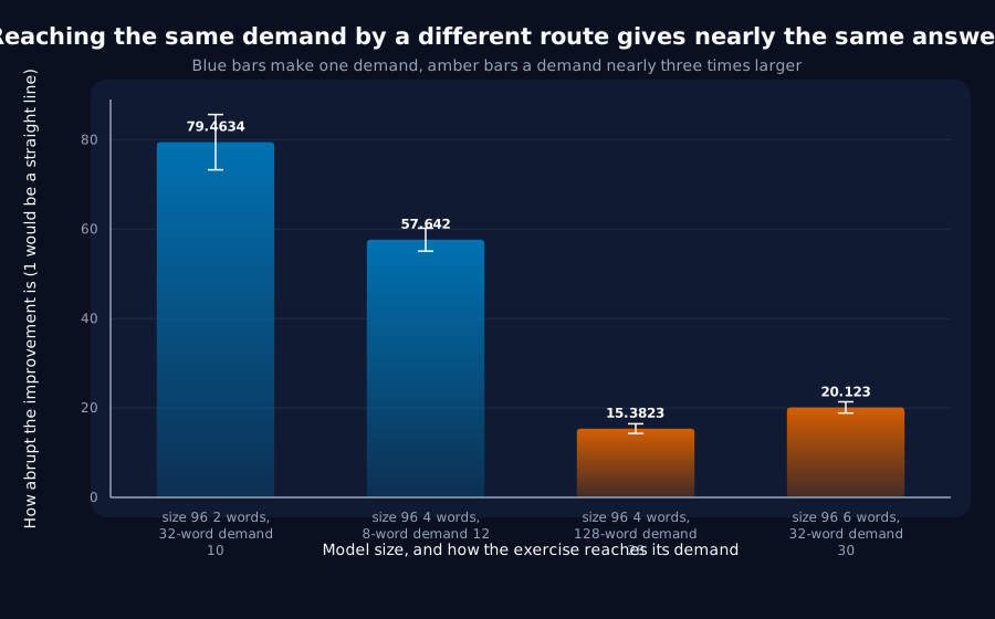
Why it matters. The half that did survive is worth as much as the half that failed, and it is the half with no adjustable numbers in it. We measure an exercise's demand as how many things the model has to hold in mind times how much information each one carries. You can reach the same total two different ways: hold fewer things drawn from a bigger vocabulary, or more things drawn from a smaller one. Settings that reach the same demand by different routes land close together, and settings at genuinely different demands land far apart, by about four to one. Afterwards, once the verdict was already fixed, we let the two ingredients trade off freely instead of forcing them to combine the way our formula says. It changed nothing: the two came out within about one percent of each other and the fit was no better. So the way we describe how hard an exercise is turns out to be right. Dividing model size by it is what does not work. The next question costs us nothing at all, because those same hundred runs already recorded something we never looked at: not how sharp each jump was, but when it happened.

The rest of this page is the technical record: the design, every number, and the limits. It is written for a reviewer, and you do not need it to have understood the result above.

New here? How to read a research record

Start at the verdict. Every record states, before the experiment was run, what result would have made us abandon the idea. That is the "kill test". Then it says whether the test fired. Nothing gets reinterpreted after the fact.
Numbers in square brackets are uncertainty. 23.4 [18.1, 28.7] means our best estimate is 23.4 and the true value is probably somewhere in that range. If a range includes zero, we cannot claim an effect.
Negative results are kept. Roughly half of what is published here says an idea did not work, including several of our own. Those pages are not failures, they are the output. Work that only publishes what worked is not measuring anything.
Read the Limits section. Every record ends with what it does not show. It is the most honest part of any experiment and usually the shortest.
Pro tip: the figures near the top are designed to carry the result on their own. If you read nothing else, read the caption under each one, which says what it shows and what to take from it.

EXPLORATORY. Not a preregistered study. Local CPU, 100 training runs, no GPU, no cost.

Program v2 Bucket N, item N6. Decisive computation: analysis/capacity_ratio.py. Output: analysis/capacity_ratio.json. Reproduce with python analysis/capacity_ratio.py, or re-derive every endpoint with --reuse.

The question

M5 found that the sharpness of the learning transition falls monotonically with width, 22.58 at width 48, 17.35 at 32, 12.70 at 24, while the model still solves the task to 0.96. M1 found the task needs essentially nothing: a zero-parameter cache solves it outright.

**Spare capacity alone does not decide how abruptly a model learns.** Each line is one exercise, run at four model sizes. The horizontal axis is spare capacity: how big the model is, divided by how much the exercise demands it hold in mind. If spare capacity were the whole story the four lines would lie on top of one another. They do not. Read straight up from 3.2: three different settings sit at that same spare capacity, and the easiest of them improves twice as abruptly as the hardest. Making the model bigger and making the exercise easier both make the improvement more abrupt, but they do not cancel out. Difficulty counts roughly twice as much as size, so you cannot describe one by dividing it into the other.

**Size and difficulty pull in opposite directions, and not equally hard.** Every combination of model size across the columns and exercise down the rows. The number in each cell is how abrupt the improvement was, where 1 would mean the model improved at a perfectly steady rate from start to finish. Reading along a row shows what a bigger model does; reading down a column shows what a harder exercise does. Both directions matter and neither can be ignored. Doubling the model's size adds about 12 to abruptness; doubling what the exercise demands takes away about 27. That imbalance is why dividing one by the other does not describe the picture.

**Reaching the same demand by a different route gives nearly the same answer.** This is the half of the test with no adjustable number anywhere in it. Two exercises can demand the same amount of remembering by different routes: hold fewer words drawn from a larger vocabulary, or more words drawn from a smaller one. The two blue bars make one demand by two routes, the two amber bars a demand nearly three times larger by two routes. Bars sharing a colour should match if the demand is what matters; bars of different colours should not. The gap between the colours is about four times the gap within them, so how much an exercise demands is a fair description of how hard it is. The route taken to that demand matters much less than the size of it.

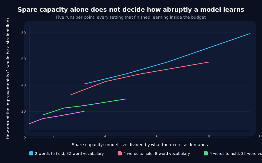
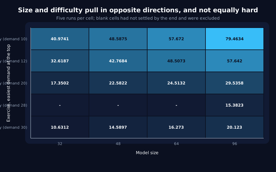
Put those two together and width is the wrong variable. The natural one is width relative to what the task requires, and in fifty-odd records this programme had never varied the requirement: every delayed-copy run in the archive uses the same lag and the same vocabulary (F10 says so explicitly). So vary both, on a grid, and ask whether the two axes collapse onto one curve in their ratio.

Kill test, fixed in advance: sharpness depends on width and difficulty separately, with no collapse.

The design

Capacity is the hidden width H, not the parameter count. A GRU's recurrent state is what has to carry the prefix; its embedding and readout are V x H, which would tie the capacity axis to the vocabulary axis, one of the two things being swept. Using H keeps the axes independent.

**Requirement is R = lag * log2(vocab) bits, with no fitted constant in it.** synthetic-delayed-copy-v1 builds each sequence by repeating a random prefix of lag tokens, so a model that has retained those lag tokens can emit every scored position and one that has not cannot. That is exactly lag * log2(V) bits.

The grid reaches the same requirement two different ways. Two pairs of settings have nearly equal R by different routes: lag2-v32 (R = 10) against lag4-v8 (R = 12), and lag4-v128 (R = 28) against lag6-v32 (R = 30), while the pairs are 2.6x apart from each other. If R is the right variable, within-pair differences at matched width are small and between-pair differences are large. That test has no free parameter in it at all, which is why it carries as much weight here as the curve fit does.

Four widths (96, 64, 48, 32) x five difficulties x five seeds, 2,500 steps each, everything else held at M5's configuration.

The controls, which is where the work is

The anchor is a precondition in code, not a number printed beside the result (K3). The lag4-v32 / width-48 cell is M5's configuration exactly: same task, seeds, steps, rate, batch and evaluation cadence, so it must reproduce M5's published sharpness and transition. The test is interval overlap, not point-in-interval (K6): an anchor that gets stricter as the replication gets better is the wrong test. If the anchor fails, no verdict is printed at all.

The settling confound runs along the hypothesis. Sharpness is the largest change as a share of the run's total change, so a curve still climbing when the run ends has a denominator that is not final and reads as gradual whether or not it is. Low-rho cells are the narrow ones on the hard tasks; they settle last; unsettledness depresses sharpness. Every cell carries M5's still-climbing check and an unsettled cell is excluded from the fits and from the verdict rather than entering them as gradual.

A flat endpoint collapses onto everything, G6's ceiling trap in another costume. The between-cell spread must exceed the seed-noise floor by 3x before any model of it is read.

The matched-pair ratio is guarded at both ends (J8's determinate denominator and K7's "a control built to be flat sits on zero"). The kill test's own world is the degenerate case: if only width matters, both cells in a pair share a width, the within-pair gap collapses to noise, the between-pair gap does too, and an unguarded ratio reads 0/0 as a pass. So the between-pair difference must clear 3x the noise floor before the ratio is read, and the within-pair difference must clear the floor at all.

Nothing here may be compared to a record that used a different budget. Sharpness is normalised by the run's own total change (N5), so every cell runs for exactly 2,500 steps.

Result: the kill test fires

The anchor reproduced before anything else was read. The lag4-v32 / width-48 cell is M5's configuration exactly, and the script refuses to print a verdict unless it reproduces:

endpoint	this run	M5 published
sharpness	`22.58` `[21.54, 23.63]`	`[21.54, 23.63]`	overlap
transition	`91.0` `[88.2, 93.8]`	`[88.0, 94.0]`	overlap

The full grid, five seeds per cell, 2,500 steps each. rho is capacity over requirement, H/R:

exercise	width	`R`	`rho`	final accuracy	sharpness	transition
lag2-v32	96	10	9.60	`1.0000`	`79.46` `[73.28, 85.64]`	`30`
lag2-v32	64	10	6.40	`1.0000`	`57.67` `[54.70, 60.65]`	`49`
lag2-v32	48	10	4.80	`1.0000`	`48.59` `[42.84, 54.34]`	`61`
lag2-v32	32	10	3.20	`1.0000`	`40.97` `[37.46, 44.48]`	`79`
lag4-v8	96	12	8.00	`1.0000`	`57.64` `[55.07, 60.22]`	`29`
lag4-v8	64	12	5.33	`1.0000`	`48.51` `[46.71, 50.31]`	`35`
lag4-v8	48	12	4.00	`1.0000`	`42.77` `[37.62, 47.92]`	`39`
lag4-v8	32	12	2.67	`1.0000`	`32.62` `[29.69, 35.54]`	`53`
lag4-v32	96	20	4.80	`0.9988`	`29.54` `[27.43, 31.65]`	`58`
lag4-v32	64	20	3.20	`0.9950`	`24.51` `[20.57, 28.46]`	`77`
lag4-v32	48	20	2.40	`0.9957`	`22.58` `[21.54, 23.63]`	`91`
lag4-v32	32	20	1.60	`0.9910`	`17.35` `[15.35, 19.35]`	`111`
lag4-v128	96	28	3.43	`0.9714`	`15.38` `[14.30, 16.46]`	`191`
lag4-v128	64	28	2.29	`0.9457`	,	, (unsettled)
lag4-v128	48	28	1.71	`0.9234`	,	, (unsettled)
lag4-v128	32	28	1.14	`0.6694`	,	, (unsettled)
lag6-v32	96	30	3.20	`0.9889`	`20.12` `[18.86, 21.39]`	`84`
lag6-v32	64	30	2.13	`0.9827`	`16.27` `[14.96, 17.58]`	`107`
lag6-v32	48	30	1.60	`0.9738`	`14.59` `[13.81, 15.37]`	`123`
lag6-v32	32	30	1.07	`0.9531`	`10.63` `[9.52, 11.75]`	`165`

The bolded row is the anchor cell. All 100 runs learned. Three cells were still climbing at step 2,500 and are excluded from every fit and from the verdict, which leaves 17 settled cells.

The clearest form of it needs no fit at all

Three cells share rho = 3.20 exactly, reached by three different combinations of width and requirement. If rho were the variable, they would agree:

`rho`	exercise	width	`R`	sharpness
3.20	lag2-v32	32	10	`40.97` `[37.46, 44.48]`
3.20	lag4-v32	64	20	`24.51` `[20.57, 28.46]`
3.20	lag6-v32	96	30	`20.12` `[18.86, 21.39]`

They span 2.0x, the extremes do not overlap, and they are ordered by R. The same happens at the other two shared values of rho: at 4.80, 48.59 against 29.54; at 1.60, 17.35 against 14.59. In all three families the higher requirement is the less abrupt, at equal rho.

The fits say the same thing with numbers on it

model of sharpness	residual RMS
width alone	`17.98`
requirement alone	`9.18`
`rho = H/R` alone	`8.89`
free slopes on width and requirement	`5.78`
seed-noise floor	`1.14`

rho barely improves on requirement alone (8.89 against 9.18), and letting the two axes take their own slopes cuts the residual by a further 35%. The preregistered tolerance was 1.5x the noise floor, or 1.70; rho's residual is 5.2x that.

The free fit says why. Sharpness moves +12.11 per doubling of width and -27.08 per doubling of requirement. Collapse in rho requires those to be equal and opposite, because log2(rho) = log2(H) - log2(R). Their ratio is 2.24, not 1.00: the requirement axis is about twice as strong as the capacity axis.

The endpoint is not flat, so this is not G6's ceiling in another costume, the between-cell spread is 19.41 against a 1.14 noise floor, 17.1x.

The parameter-free half passes, and it is worth separating from the headline

The matched pairs reach near-equal requirements by different routes. Only width 96 has all four cells settled, so the comparison rests on that width:

		sharpness
pair 1 (`R = 10`)	lag2-v32	`79.46`
pair 1 (`R = 12`)	lag4-v8	`57.64`
pair 2 (`R = 28`)	lag4-v128	`15.38`
pair 2 (`R = 30`)	lag6-v32	`20.12`

Between-pair 50.80, within-pair 13.28, ratio 3.83 against a floor of 3.0, with both halves clearing their guards: 50.80 clears 3x the noise floor, and 13.28 clears it too, so the denominator is a difference rather than 0/0.

The two halves of the test therefore point in different directions, and both are reported: R is a fair description of an exercise's difficulty; H/R is not a fair description of the pair.

Post hoc, and it decides nothing above

The within-pair gaps are large enough to ask whether R = lag * log2(V) prices a lag token and a vocabulary doubling at the right rate against each other. Splitting R back into its ingredients is the cheapest test of that, and it was computed after the verdict was already fixed:

model	residual RMS	slopes
width and `R`, the bit-count imposed	`5.78`	width `+12.11`, `R` `-27.08`
width, lag and vocabulary bits, all free	`5.78`	width `+12.08`, lag `-27.17`, vocab bits `-26.81`

Freeing the exchange rate buys nothing. The two ingredient slopes land within 1.3% of each other and the residual does not move, which is exactly what R = lag * log2(V) asserts. The bit-count is doing its job; the division by it is what fails.

The signed pairs go 4/5 with the bit-count's own ordering. The exception is lag4-v128 against lag6-v32 at width 96 (-4.74, non-overlapping intervals), where the cell needing more bits is the more abrupt of the two, the same cell family that failed to settle at every narrower width.

Verdict

The kill test fires. Width and difficulty act separately. Sharpness does not collapse onto one curve in H/R: the residual is 8.89 against a 1.70 tolerance, and rho scarcely improves on requirement alone.
The anchor reproduced as a precondition in code, on M5's exact configuration, seeds and budget.
Three cells at identical rho span 2.0x in sharpness with non-overlapping extremes, which is the finding with no fit in it.
The two axes have different strengths: +12.11 per doubling of width against -27.08 per doubling of requirement, a ratio of 2.24 where collapse needs 1.00.
The requirement is nonetheless the right difficulty variable. The parameter-free matched-pair ratio is 3.83, and freeing the lag/vocabulary exchange rate post hoc changes the residual by nothing.
The endpoint varies 17.1x its noise floor, so the verdict is not a ceiling effect.
--reuse reproduced the whole JSON bit-for-bit, verdict and cells identical.

Limits

The matched-pair test rests on one width. lag4-v128 never settled below width 96, so the between/within comparison has a single width behind it. The 3.83 is one number, not an interval over four.
Unsettled cells are excluded, and they are not excluded at random. They are the narrow cells on the hardest exercise, exactly the low-rho corner the hypothesis most wanted read. Excluding them is the honest handling of an endpoint normalised by a run's own total change (N5), but it means the rho range tested runs 1.07 to 9.60 with a hole in the hardest corner. A longer budget would fill it, and that is the obvious follow-up.
Capacity here is the hidden width, not the parameter count. That choice keeps the capacity axis independent of the vocabulary axis, and it means nothing here speaks to parameter count as such.
The requirement has no fitted constant, which is both a strength and a restriction. lag * log2(V) is what synthetic-delayed-copy-v1 demands by construction. A task whose demand is not countable that way has no R to divide by, and this result does not say what to use instead.
2.24 is a slope ratio from a semi-log fit over 17 cells, not a law. It says the axes are unequal and roughly by how much; it does not establish the functional form.
One architecture, one optimiser, one learning rate, one budget, five seeds. Sharpness is normalised by the run's own total change, so nothing here may be compared against a record run for a different number of steps.
This is an offline description, not an instrument. It says what sets abruptness, not how to detect it while training, and this programme has repeatedly found that a real signal still has to be priced against what detecting it costs (J7).

Terms on this page

Every piece of vocabulary this record uses, in plain language. Generated from the text above, so it cannot drift out of step with it.

accuracy: The fraction of answers a model gets right on questions it was not trained on.
architecture: The blueprint of a model: what components it has and how they connect. Two models can be the same size and completely different architectures.
confound: A second explanation you did not control for. If bigger models both learn faster and score higher, then 'fast learners score higher' may be entirely about size and not about speed.
GRU: Gated Recurrent Unit. A compact design for processing sequences one item at a time, with internal switches controlling what it keeps in memory.
kill test: A condition written down before running the experiment that says what result would make us abandon the idea. Fixing it in advance is what stops a disappointing result being reinterpreted as an encouraging one.
learning rate: How big a step training takes each time it updates the model. Too small and nothing happens; too big and it never settles.
noise floor: How much a measurement wobbles between repeats of the identical setting. Any difference smaller than this is indistinguishable from luck, so it is the reference point every other number here is judged against.
post hoc: Worked out after the fact, rather than decided in advance. We report such checks separately and never let them decide a result, because it is far too easy to find a pattern once you already know the answer.
recurrent: A design that reads a sequence one item at a time, carrying memory forward. The main alternative is attention, which looks at everything at once.
residual: How far the data sits from a proposed description of it, after the description has been fitted as well as it can be. A small residual means the description accounts for what was measured; a large one means something is missing.
seed: The number that fixes all the randomness in a training run. Same seed, same run. Running several seeds is how you tell a real effect from a lucky one.
sharpness: How abrupt a model's improvement is. We measure the biggest change over any short stretch of training as a share of the run's total change, scaled so that a model improving at a perfectly steady rate would score 1. A score of 20 means the fastest stretch was twenty times steeper than a straight line.
slope: How steeply one quantity changes as another does. A slope of one between a warning and the event it predicts means the warning shifts exactly in step with the event.
vocabulary: The set of distinct symbols a model can read and produce.
width: How many internal numbers a model uses at each layer. The usual way we vary model size in these experiments.