Predicting It Without Watching

Ongoing research. This is an experimental result from active work, not a settled conclusion. The numbers are what we measured and the method is described so you can judge it, but the programme is still running and later experiments may revise what it means. More about this programme.

In plain English

What we asked. Models in these experiments do not improve steadily. They flounder for a while, then get much better very quickly over a short stretch, then level off. Knowing when that moment will arrive is genuinely useful, because anything you might want to do about it has to be done before it happens. We have one instrument that gives warning, and it works: it watches the run as it goes and raises a flag about 23 steps before the improvement. It is also the most expensive thing we own, adding 55 percent to the cost of training. This project has a standing rule that an instrument has to be measured in the same units as the benefit it buys, and we had never applied that rule to this instrument against the obvious free alternative: just working out in advance, from runs you have already done, when the moment is likely to be.

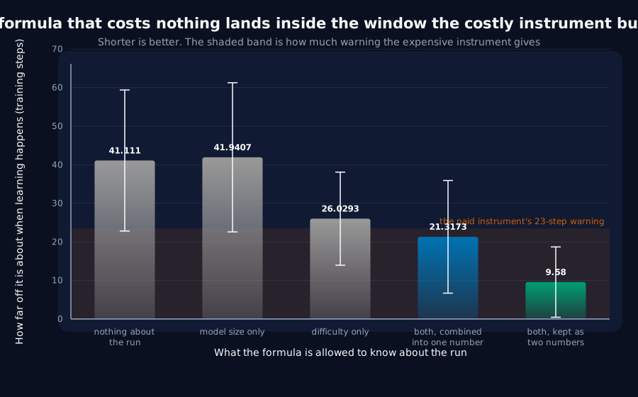
What we found. The comparison needed no new training at all. A hundred runs we had already done recorded when each one improved, and nobody had ever fitted anything to that column. So we fitted a formula to it, and tested it the honest way: fit on sixteen settings, predict the seventeenth, which the formula has never seen. Told only how big the model is, the formula predicts nothing useful once the exercise is allowed to vary too. Told the size and the difficulty combined into a single number, it lands about 21 steps off, which is inside the paid instrument's window on average but with too much uncertainty to call either way. Told the size and the two ingredients of difficulty as separate numbers, it lands 9.6 steps off, comfortably inside the window, and it does that on 16 of the 17 settings. So the answer is yes: something free can do what the expensive thing does, on the settings we can test.

Why it matters. The interesting part is why the combined version fails. An earlier result of ours checked that same way of combining difficulty into one number and found it exactly right, and we trusted it here. It is right, but only about one thing. It correctly describes how abruptly a model improves, and it gets the timing wrong by a factor of three, because a bigger vocabulary delays the moment far more than the formula says it should. A description that has been checked against one property of an event does not automatically describe another property of the same event, which is worth knowing anywhere a single number is being used to stand in for how hard something is. Two things belong beside the headline. If you ask which instrument names the exact moment more accurately rather than which gives more notice, the paid one still wins, and it turns out to need calibration runs of its own to do it. And the whole comparison depends on where you draw the finishing line for 'has learned it': the free formula wins at the line we published and every easier one, and loses at the strictest ones. We swept it and showed the reversal rather than reporting the number that suited us.

The rest of this page is the technical record: the design, every number, and the limits. It is written for a reviewer, and you do not need it to have understood the result above.

New here? How to read a research record

• Start at the verdict. Every record states, before the experiment was run, what result would have made us abandon the idea. That is the "kill test". Then it says whether the test fired. Nothing gets reinterpreted after the fact.
• Numbers in square brackets are uncertainty. 23.4 [18.1, 28.7] means our best estimate is 23.4 and the true value is probably somewhere in that range. If a range includes zero, we cannot claim an effect.
• Negative results are kept. Roughly half of what is published here says an idea did not work, including several of our own. Those pages are not failures, they are the output. Work that only publishes what worked is not measuring anything.
• Read the Limits section. Every record ends with what it does not show. It is the most honest part of any experiment and usually the shortest.
• Pro tip: the figures near the top are designed to carry the result on their own. If you read nothing else, read the caption under each one, which says what it shows and what to take from it.

EXPLORATORY. Not a preregistered study. Local CPU, no training at all, no GPU, no cost.

Program v2 Bucket N, item N14. Decisive computation: analysis/schedule_versus_probe.py. Output: analysis/schedule_versus_probe.json. Reproduce with python analysis/schedule_versus_probe.py in about two seconds: it re-analyses three committed pilot outputs and trains nothing.

The question

F2 is this programme's only positive instrument. A linear probe fitted from the hidden state to the token the model should emit crosses 50% accuracy about +23.5 steps before the model's own accuracy does, on a transition that lands near step 85. It is also the most expensive thing here: J7 measured running it at 55.4% of the training budget, thirteen times the saving it bought when it was acted on.

There has always been a free alternative and it had never been priced against the probe. E4 established half of it, transition step falls with width by 7.4x more than seed noise, giving ±10-step scheduling precision, and E4's own record calls this "an offline schedule, not an online leading indicator". N6 then ran a grid crossing width with difficulty, and its 17 settled cells each carry a transition step that N6 never fitted. Put the two together and the comparison this programme's method demands becomes possible for the first time:

a formula costing nothing, fitted on 16 cells, predicting the 17th against a probe costing 55.4% of the budget, reading the run in front of you

Why an error and a lead are comparable. To act X steps before the transition you have to know where it is to better than X. The probe buys +23.5 steps of notice; a schedule that localises the event to ±E steps buys the same notice for nothing as long as E is smaller. The two numbers are in the same units and answer the same operational question, which is exactly the pricing J7 made this programme's standing rule.

Kill test, fixed in advance in docs/research-program-v2.md: the leave-one-out prediction error exceeds 23.5 steps. Also killed if the error is dominated by the seed-to-seed spread of the transition itself, in which case neither instrument resolves anything.

The design, and the two things it had to get right

Both instruments must time the same event. F2 and J5 time an absolute accuracy crossing at 0.5; N6 times a floor-to-ceiling midpoint. Those are different events, and a floor-to-ceiling midpoint additionally is not comparable across runs of different lengths (N5), which bites here, because N6 runs 2,500 steps and J5 runs 900. So the head-to-head uses the absolute crossing, which has no length dependence once the curve reaches the level, and N6's midpoint appears only in the anchor.

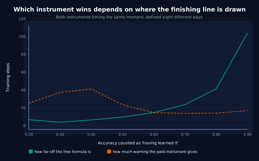
The crossing level is then swept 0.2 to 0.9. A comparison with a free parameter fixed at one value cannot be told from a comparison tuned to that value, G6's ceiling trap in another costume. The sweep turned out to matter: see below.

One premise in the backlog item was wrong and is corrected here. The item asks for "K4's warm-up" to be charged to the probe. K4's 41-step warm-up belongs to K1's gradient alarm, a 20-step rolling window plus the median history it is thresholded against, and not to the decode probe, which has no rolling window at all. The probe's own timing constraint is different in kind, and J5 measured it: its crossing races earlier as models widen, reaching step 5.5 of a 34-step run at width 192. J5's measurement is used below in place of K4's number.

The controls

Two anchors, as preconditions in code rather than numbers printed beside the result (K3), one per side of the comparison, both interval-overlap tests rather than point-in-interval (K6):

anchor	this file	published
N6's lag4-v32/width-48 cell, midpoint definition	91.0 [88.2, 93.8]	[88.0, 94.0] (M5)	overlap
J5's width-48 curves, re-timed here by this file's own crossing function	+23.53 [+20.49, +26.57]	[+22.08, +24.87] (F2)	overlap

Every error is leave-one-out, so a fit with more freedom cannot win by construction. The ladder was fixed before running: the grand mean, width alone (E4's half), requirement alone, both (N6's contribution), and a fifth rung that splits the requirement back into lag and log2 V with free slopes.

Leaving one cell out is the easy version of the question, so two harder splits are reported beside it: leave a whole difficulty out (can the schedule place the transition for a task nobody has run?) and leave a whole width out.

The seed spread of the event is the reference point. Both instruments are trying to resolve it.

What the formula needs that the probe does not, stated rather than left implicit: its coefficients come from other runs. It is a schedule transferred across cells of one family, one architecture, one optimiser, one learning rate, not a reading of the run in front of you.

Result: the kill test does not fire, and the interval says why that is only half an answer

Seventeen settled cells, five seeds each, timing a 50% crossing. The seed spread of the event itself is 5.0 steps (standard error of a cell mean 2.2; evaluation resolution 5), so both instruments are working well above the noise and the second kill-test condition does not apply.

model of the transition step	cell-mean error	median	inside the 23.5-step lead
grand mean (no predictors)	41.1 [22.8, 59.4]	35.3	7/17
width alone (E4's half)	41.9 [22.6, 61.3]	36.7	6/17
requirement alone	26.0 [14.0, 38.1]	22.1	10/17
width and requirement	21.3 [6.7, 35.9]	17.3	15/17
width, lag and vocabulary, free slopes	9.6 [0.5, 18.7]	5.3	16/17
(fitted linear in steps rather than as a power law)	27.9 [15.7, 40.1]

At the letter of the kill test it does not fire: 21.3 < 23.5. But this programme requires the interval rather than the point estimate, and [6.7, 35.9] spans the probe's lead, so the bit-count form is undecided: it cannot be said to reach the probe's window or to miss it.

The form that does decide it is the one that stops compressing difficulty into a single number. Freeing the exponents on lag and log2 V gives 9.6 steps [0.5, 18.7], an interval lying entirely inside the probe's lead, with 16 of 17 settings localised inside it. The median error is 5.3 steps, one evaluation interval.

Width alone is worse than nothing. 41.9 against the grand mean's 41.1: across a grid that varies difficulty, E4's half of the schedule on its own carries no usable information at all. That is not a contradiction of E4, which held difficulty fixed; it is the measurement of how much of the schedule the difficulty half supplies.

The fitted schedule, and the exchange rate that decides it

	fitted on all 17 cells
bit-count form	T = 2^3.95 · H^-0.591 · R^1.316
free form	T = 2^2.57 · H^-0.696 · lag^0.846 · (log2 V)^2.637

R = lag · log2 V prices a lag token and a vocabulary doubling at the same rate. Freed, their exponents are +0.846 and +2.637, vocabulary costs 3.12x what the bit-count says it does.

This is the part worth carrying, because N6 ran the same check on sharpness and got the opposite answer. There, freeing the exchange rate bought nothing: the two ingredient slopes landed within 1.3% of each other and the residual did not move, which is what R = lag · log2 V asserts. The same bit-count is a fair description of difficulty for how abrupt the transition is and a wrong one for when it happens. A difficulty measure validated on one endpoint does not transfer to another endpoint of the same event.

The single cell that carries the bit-count's error is lag4-v128 at width 96, predicted at step 66 against an actual 192. Its whole column failed to settle at every narrower width, so it is the only settled cell at that vocabulary, which means leaving it out leaves the fit with no run at that vocabulary at all, and its prediction is an extrapolation in exactly the variable the bit-count misprices. Dropping it leaves 14.8 steps for the bit-count and 5.5 for the free form. The headline numbers above include it.

The harder splits: a task nobody has run

model	leave one difficulty out	leave one width out
grand mean	47.4 [28.6, 66.2]	39.8 [22.0, 57.7]
width alone	47.5 [27.9, 67.2]	38.8 [19.3, 58.3]
requirement alone	31.1 [20.1, 42.1]	26.0 [15.4, 36.6]
width and requirement	32.8 [17.7, 47.9]	19.1 [4.1, 34.1]
width, lag and vocabulary	14.5 [5.8, 23.1]	9.1 [0.1, 18.1]

Predicting a difficulty the fit has never seen costs the free form 9.6 → 14.5 steps, and its interval still ends just inside the probe's lead (23.1 against 23.47). Predicting an unseen width costs almost nothing. Interpolating across sizes is close to free; extrapolating across tasks is where a schedule is fragile, which is the ordering a practitioner should expect and the opposite of the one this programme's width-only history would have suggested.

The probe, scored the same way

The probe does not name a step, it fires. To put both instruments in the same units it is turned into a predictor: its own crossing plus the mean lead of the other runs, leave-one-out, on J5's saved curves, at the same crossing level. The conversion is deliberately generous: the lead is calibrated at the same width.

width	transition	probe fires at	lead	error as a step predictor
16	323.5	301.6	+21.9	4.7
32	108.8	94.0	+14.8	1.5
48	85.2	61.6	+23.5	2.4
96	52.5	15.5	+37.0	1.9
192	33.9	5.5	+28.4	0.9

As a predictor of the step, the probe is the more accurate instrument: 2.3 steps [1.2, 3.4] overall against the free schedule's 9.6. Two things belong beside that number and neither is in the probe's favour:

• It needs a calibration set too. Converting an alarm into a predicted step requires knowing the lead, and the lead is not a constant, J5 measured it from +14.8 to +37.0 across widths. Given one lead for every width instead of a same-width one, the probe's error goes to 7.0 steps [5.3, 8.8]. The asymmetry the comparison started with is smaller than it looks: both instruments are calibrated from other runs, and only one of them also costs 55.4% per run.
• Width-matched, at the configuration where the probe was measured (lag4-v32, widths 32, 48, 96), the free schedule is at 2.9 steps against the probe's 1.9. With the whole lag4-v32 column held out, so the fit has seen no run at that difficulty, the bit-count form is at 3.4 steps and the free form at 12.9.

The crossing level, swept

Both instruments have the same free parameter, and the answer depends on it:

level	free schedule's error	bit-count's error	probe's lead at width 48
0.2	6.7	8.2	+25.4
0.3	3.8	16.7	+37.3
0.4	6.5	19.5	+41.2
0.5	9.6	21.3	+23.5
0.6	14.8	23.5	+14.6
0.7	23.7	31.1	+13.9
0.8	41.5	49.6	+14.1
0.9	104.0	112.9	+16.8

The ordering reverses at 0.6. Read row by row, both instruments timing the same event at the same level, the free schedule's error is inside the probe's own lead at 0.2 through 0.5, ties it at 0.6 (14.8 against 14.6) and is outside it from 0.7 on. Timing a low crossing is easy to predict and gives the probe a long lead; timing a high one is the tail of saturation, which no formula in width and difficulty predicts, while the probe tracks it because both curves saturate together. The published 0.5 is not the level most favourable to the schedule (0.3 is), and quoting any single level would have hidden the reversal entirely.

Cost, in the same units as the benefit

	cost
probe	55.4% of every run it watches, for ever (J7)
schedule	nothing per run; 80 calibration runs of 2,500 steps, paid once
break-even	the calibration costs what the probe costs after 144 runs of the same length

An unplanned cross-check that passed

E4 fitted T ~ width^-0.615 on the committed archive: different widths (36, 48, 72), a different event definition, other seeds, a different budget. This grid's lag4-v32 column gives -0.640. Nothing was tuned to make that happen and it decides nothing here, but two independent estimates of the same exponent landing 4% apart is the strongest evidence this programme has that the width scaling is a property of the task rather than of one pilot.

Verdict

• The kill test does not fire. The leave-one-out error of the two-variable formula is 21.3 steps against the probe's +23.5-step lead. Its interval [6.7, 35.9] spans the lead, so the bit-count form is undecided, and reporting the point estimate alone would have overstated it.
• The free form decides it: 9.6 steps [0.5, 18.7], entirely inside the lead, 16/17 settings localised inside it, median error 5.3 steps. A schedule costing nothing per run reaches the window the 55.4% instrument buys: at the published crossing level and at every lower one, with the ordering reversing at 0.6 and above.
• The second kill-test condition does not apply. The event's own seed spread is 5.0 steps, well inside both instruments' resolution.
• The bit-count that N6 validated for sharpness misprices timing by 3.12x. A difficulty measure that works for one endpoint of an event does not transfer to another endpoint of it.
• Scored as a step predictor rather than as an alarm, the probe is more accurate, 2.3 steps with same-width calibration, 7.0 with one lead for all widths, against the schedule's 9.6. Both instruments are calibrated from other runs; one of them also costs 55.4% per run.

Limits

• Every number is a re-analysis of runs that already existed. Nothing new was trained, so this inherits every limit of N6, F2 and J5: one architecture (a one-layer GRU), one optimiser (AdamW), one learning rate (0.005), one task family (synthetic-delayed-copy-v1), widths 32–96.
• The schedule is fitted where the probe is not measured, and vice versa. N6's grid varies difficulty at four widths; J5's sweep varies width at one difficulty. They meet at three cells. The probe's behaviour on lag4-v128 or lag6-v32 is untested, not negative, measuring it would cost roughly 85 runs at 55.4% overhead, and it is written into the backlog as N17.
• lag4-v128 settled at one width only, so the vocabulary exponent rests on a single settled cell at that vocabulary and the grid cannot say whether 2.637 is the exponent or an artifact of that corner. N18 in the backlog is the cheap fix: run the three unsettled cells longer.
• The comparison is between a lead and an error, which are different quantities that happen to answer the same operational question. A reader who wants "how accurately does each instrument name the step" should read the predictor table, where the probe wins; a reader who wants "how much notice can I get for free" should read the ladder, where the schedule reaches the probe's window.
• Leave-one-out over 17 cells with two or three parameters is a small-sample procedure. The intervals are wide and are quoted for that reason.
• The vocabulary axis is confounded with parameter count, and this was noticed in the review after publication rather than in the design. N6 chose hidden width H as capacity precisely to keep the capacity and vocabulary axes independent, but a GRU's embedding and readout are both V x H, so at width 48 the model has 14,976 parameters at V = 8, 17,280 at V = 32 and 26,496 at V = 128. That is a 77% increase across the vocabulary sweep with the recurrent state unchanged. "A larger vocabulary delays the transition by more than the bit-count says" and "a larger readout takes longer to train" both fit this data, and nothing here separates them. The headline exponent ratio of 3.12x is stated against log2 V and should be read as such until the separation is run. N19 in the backlog is the decisive test and it is cheap: allocate the slots of a large vocabulary but draw symbols from a small one, which holds the parameter count fixed while changing the difficulty.

What this feeds

• The offline schedule is now the programme's cheapest usable timing instrument and the first one whose accuracy is stated with an interval. Any future "do X near the transition" experiment has a zero-cost way to place its window, with a random-time-matched arm still required.
• N15 becomes more valuable, not less. It asks whether N6's sharpness exponents survive being measured without a threshold. This record has now shown that N6's difficulty measure fails on a different endpoint of the same event, which is a second reason to check how far that measure's validity extends.
• Two new items, both written into docs/research-program-v2.md: N17 (measure the probe's lead across the difficulty grid, so the two instruments are compared on the same cells rather than at their intersection) and N18 (settle the lag4-v128 column so the vocabulary exponent rests on more than one cell).

Terms on this page

Every piece of vocabulary this record uses, in plain language. Generated from the text above, so it cannot drift out of step with it.

accuracy

The fraction of answers a model gets right on questions it was not trained on.

AdamW

A widely used training algorithm that adapts how big a step it takes for each individual parameter. The default in most modern AI training.

architecture

The blueprint of a model: what components it has and how they connect. Two models can be the same size and completely different architectures.

calibration

Working out an instrument's settings from runs whose answer you already know, so it can be used on a run whose answer you do not.

exponent

The number in a power law that says how strongly one quantity responds to another. A bigger exponent means a steeper response to the same doubling.

extrapolation

Using a fit outside the range of the data it was built from, which is where fits are least trustworthy and where their errors are largest.

gradient

The direction and amount by which each of a model's internal numbers should change to do slightly better. Training is repeatedly following it.

GRU

Gated Recurrent Unit. A compact design for processing sequences one item at a time, with internal switches controlling what it keeps in memory.

hidden state

The model's working memory: the internal numbers it carries from one step of a sequence to the next.

kill test

A condition written down before running the experiment that says what result would make us abandon the idea. Fixing it in advance is what stops a disappointing result being reinterpreted as an encouraging one.

learning rate

How big a step training takes each time it updates the model. Too small and nothing happens; too big and it never settles.

leave-one-out

A way of testing a rule fitted to data: leave one measurement out, fit the rule on the rest, and see how well it predicts the one you held back. It stops a rule from being graded on the data it was built from.

linear probe

A deliberately simple readout attached to a model's internals to test what information is present in them. Kept simple on purpose: if something complicated can extract the answer, the complicated thing may be doing the work itself.

parameters

The adjustable numbers inside a model. Training is the process of setting them. Model size is usually quoted as a count of these.

power law

A relationship where one quantity changes by a fixed percentage whenever another one doubles, rather than by a fixed amount. Most scaling results in AI are stated this way.

probe

A small separate model trained to read information out of a bigger model's internals, used as a measuring instrument rather than as a product.

recurrent

A design that reads a sequence one item at a time, carrying memory forward. The main alternative is attention, which looks at everything at once.

residual

How far the data sits from a proposed description of it, after the description has been fitted as well as it can be. A small residual means the description accounts for what was measured; a large one means something is missing.

seed

The number that fixes all the randomness in a training run. Same seed, same run. Running several seeds is how you tell a real effect from a lucky one.

sharpness

How abrupt a model's improvement is. We measure the biggest change over any short stretch of training as a share of the run's total change, scaled so that a model improving at a perfectly steady rate would score 1. A score of 20 means the fastest stretch was twenty times steeper than a straight line.

slope

How steeply one quantity changes as another does. A slope of one between a warning and the event it predicts means the warning shifts exactly in step with the event.

vocabulary

The set of distinct symbols a model can read and produce.

width

How many internal numbers a model uses at each layer. The usual way we vary model size in these experiments.

---

Get new results as we publish them

Roughly monthly, one finding per email, in plain English first. Including the experiments that went against us, which are usually the useful ones. No sales email.

Leave this empty Email address Subscribe

Double opt-in: we send a confirmation link and add nobody who does not click it. One-click unsubscribe on every email.